Results
Contents
6. Results
During the WHOTS-16 cruise (WHOTS-16 mooring deployment, October 4-12, 2019), a weakening front north of the Hawaiian Islands acted to weaken trades across the region. This ridge to the north was eroding due to a weakening cold front north of the ridge, which led to a downward trend in winds. The front continued to weaken and sink southward through the weekend, keeping the winds light and variable. Regular trades returned by mid-week. On October 10, winds in the morning increased to 25 kt gusting to 35 kt, and there was a brief rain event in the morning. Waves during the week were also low, with a small swell from the north arriving mid-week.
Near-surface currents were almost 1 kt northward during transit to Station ALOHA, turning southward upon arrival to Station ALOHA. Eventually, the current shifted due north again, became somewhat weaker (about 0.5 kt), and remained for approximately five days. There was a nearly low sea level just to the east of Station ALOHA, not quite a fully formed eddy; it was reflected by northward flow to the east and southward flow to the west. A combination of internal semi-diurnal and diurnal tides and near-inertial oscillations was noticeable, especially in vertical shear.
Conditions during the WHOTS-16 deployment on October 5 were favorable, with light NNE winds of ~ 5 kt increasing to up to 10 kt by the end of the deployment. There were clear skies and no precipitation in the region, and 1.0 to 1.5 m waves from the east, with a strong surface current towards ENE.
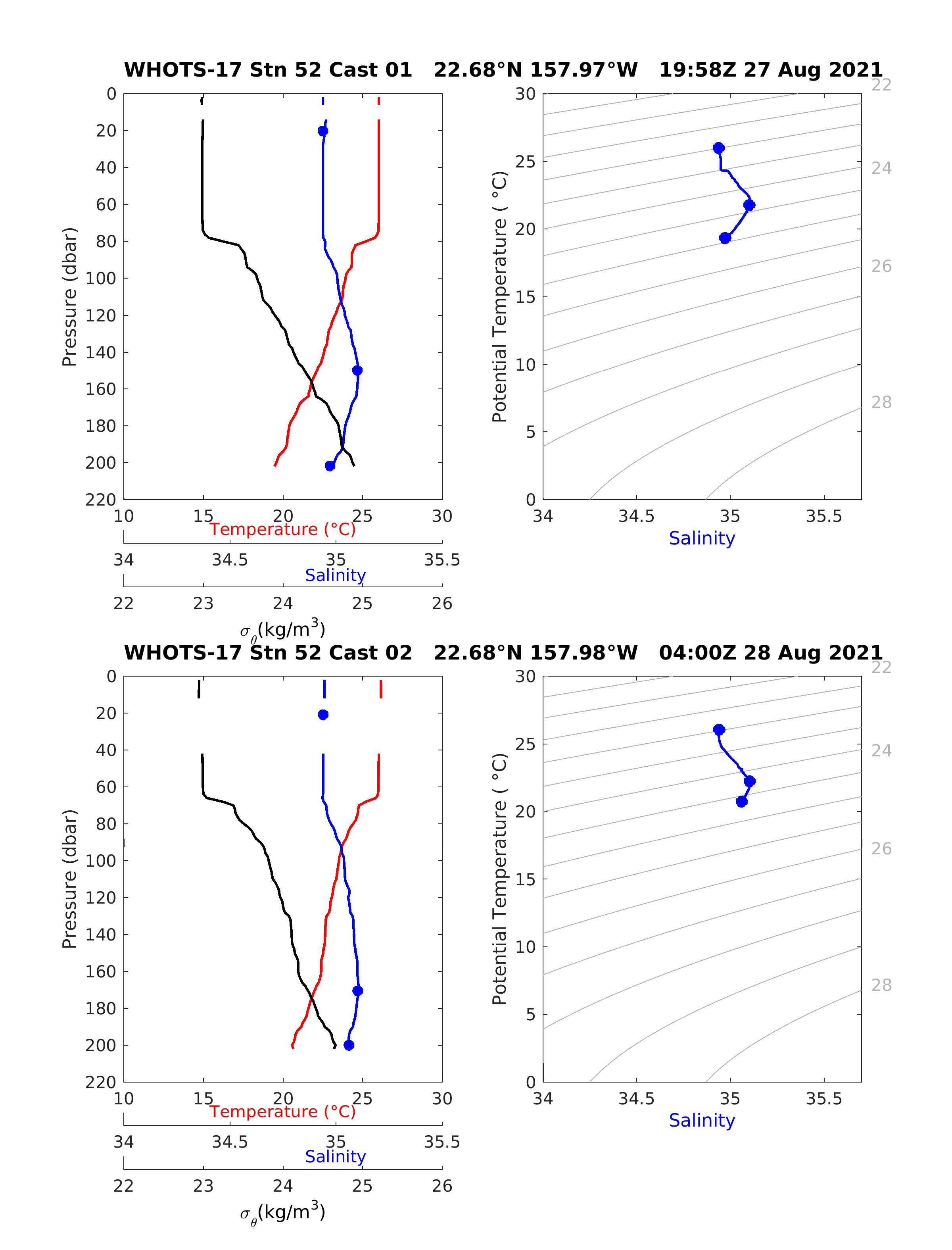
CTD casts conducted near the WHOTS-16 buoy (Station 52) after deployment (Fig. 6.4 and Fig. 6.5) displayed a subsurface salinity maximum between 70 and 80 dbar and a mixed layer 40 to 60 dbar deep.
During the WHOTS-17 cruise (WHOTS-16 mooring recovery, August 24 - September 1, 2021), a high-pressure ridge far north of the Hawaiian Islands maintained a tight enough pressure gradient down across the region to produce moderate to locally strong trades. As this high slowly moved northeast away from the area and subtly weakened the gradient, trades gradually weakened. There was no measurable precipitation during the mooring recovery, and surface currents were less than 1 kt.
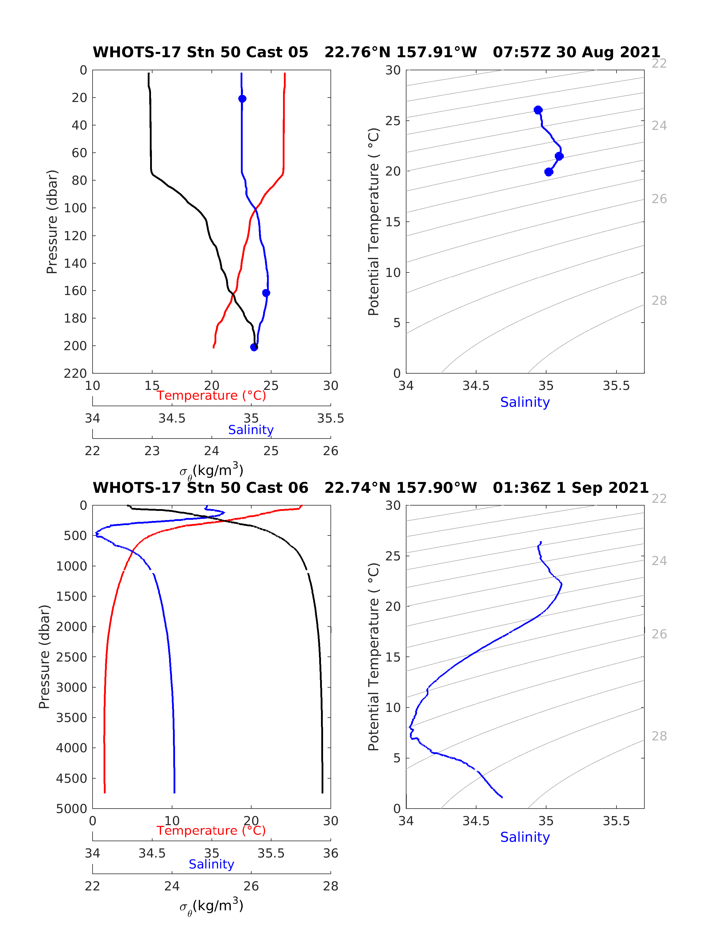
CTD casts conducted near the WHOTS-16 buoy (Station 52) before recovery (Fig. 6.10) displayed a subsurface salinity maximum between 150 and 170 dbar and a mixed layer 60 dbar deep.
The temperature MicroCAT records during the WHOTS-16 deployment (Fig. 6.15 through Fig. 6.20) show noticeable seasonal variability in the upper 100 m. A temperature decrease in October-November 2019 was evident in the instruments below 65 m. The salinity records (Fig. 6.21 through Fig. 6.26) do not show an apparent seasonal cycle, but a salinity increase was recorded during October-November 2019, by the instruments between 40 and 85 m, coinciding with the temperature decrease. This increase was followed by a period of low salinity (less than 35 on average above 120 m) throughout 2020-2021, with extreme values (nearly 34.4) above 120 m in November-December 2019, and above 75 m in July-September 2020.
Fig. 6.33 through Fig. 6.35 show contours of the WHOTS-16 MicroCAT data in context with data from the previous 15 deployments. The seasonal cycle is evident in the temperature record, with record temperatures (higher than 26°C) in the summer of 2004, and again in 2014, 2015, 2017, 2019, and 2020. Salinities in the subsurface salinity maximum were relatively low during the first 6 years of the record, only to increase drastically after 2008 through 2015, with some lower salinity episodes in mid-2011 and early 2012. The salinity maximum extended to near the surface in early 2010, 2011, late2012-early 2013, and February-March 2013. Salinities in the salinity minimum decreased after 2015, showing low salinities above 100 m in 2016, 2017, 2018, and reaching record low values (34.4) in July-August 2019 and July-September 2020. When plotted in \(\sigma\theta\) coordinates (Fig. 6.35), the salinity maximum seems to be centered roughly between 24 and 24.5 \(\sigma\theta\).
Records from the WHOTS-16 MicroCATs (Fig. 6.36) deployed near the bottom of the mooring (4713 m) detected temperature and salinity changes related to episodic ‘cold events’ apparently caused by bottom water moving between abyssal basins [Lukas et al., 2001]. These events are being monitored by instruments at the ALOHA Cabled Observatory (ACO) [Howe et al., 2011] , a deep water observatory located at the bottom of Station ALOHA (about 6 nautical miles north from the WHOTS-16 anchor), since June 2011. Fig. 6.36 shows temperature and salinity records from the WHOTS-16 MicroCATs superimposed on the ACO data. The MicroCAT data agreed with the temperature decrease and the salinity variability registered by ACO instruments during cold events in January, March and December 2020, and a minor events in August 2020 and September 2021.
Fig. 6.39 through Fig. 6.41 shows the time series of the zonal, meridional, and vertical currents recorded with the moored ADCPs during the WHOTS-16 deployment. Fig. 6.37, through Fig. 6.38, shows the ADCP current components’ contours in context with data from the previous deployments. Despite the gaps in the data, an apparent variability is seen in the zonal and meridional currents, apparently caused by passing eddies. There have been periods of intermittent positive or negative zonal currents on top of this variability, for instance, during 2007-2008. The contours of the vertical current component Fig. 6.38 show a transition in the magnitude of the contours near 47 m, indicating that the 300 kHz ADCP located at 126 m moves more vertically than the 600 kHz ADCP located at 47.5 m.
A comparison between the moored ADCP data and the shipboard ADCP data obtained during the WHOTS-16 cruise is shown in Fig. 6.42, and Fig. 6.43, and a similar comparison during the WHOTS-17 cruise is shown in Fig. 6.44 and Fig. 6.45. Some differences were seen, especially in the zonal component, maybe due to the mooring motion, which was not removed from the data. Comparisons between the available shipboard ADCP from HOT-316 to -332 cruises and the mooring data are shown in Fig. 6.46 through Fig. 6.49.
The Xeos-GPS receiver registered the WHOTS-16 buoy motion, and its positions are plotted in Fig. 6.51. The buoy was located west of the anchor for most of the deployment, except from around June to November 2020, when it was east. The power spectrum of these data (Fig. 6.51) shows extra energy at the inertial period (~31 hr). Combining the buoy motion with the tilt (a combination of pitch and roll) from the ADCP data (Fig. 6.53) showed that the tilt increased as the buoy distance from the anchor WHOTS-16 increased. This was expected since the inclination of the cable increases as the buoy moves away from the anchor.
6.1. CTD Profiling Data
Profiles of temperature, salinity, and potential density (\(\sigma\theta\)) from the casts obtained during the WHOTS-16 deployment cruise are presented in Fig. 6.1 through Fig. 6.5, together with the results of bottle determination of salinity. Fig. 6.6 through Fig. 6.10 shows the results of the CTD profiles during the WHOTS-17 cruise.
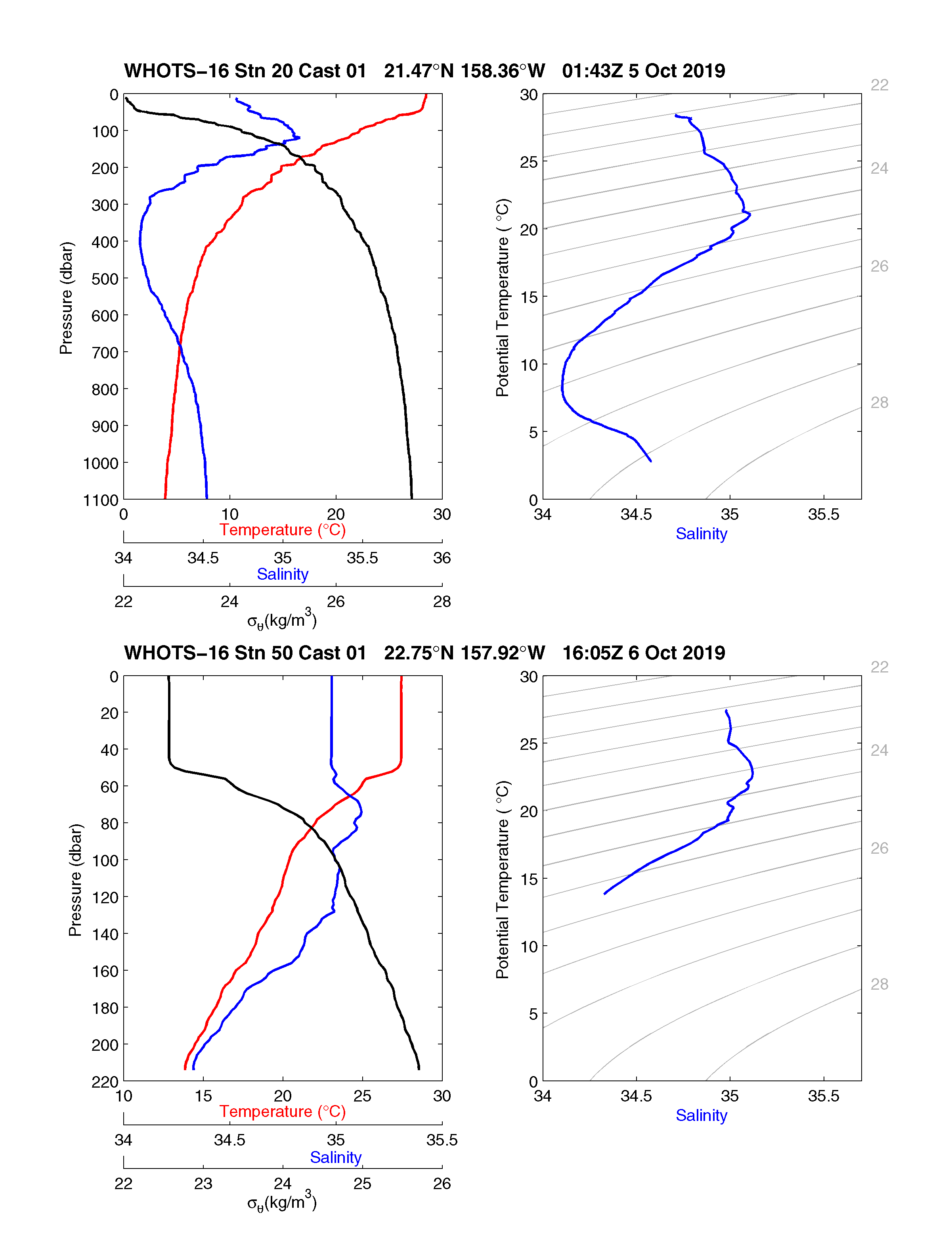
Fig. 6.1 [Upper left panel] Profiles of CTD temperature, salinity, and potential density (\(\sigma\theta\)) as a function of pressure, including discrete bottle salinity samples (when available) for station 20 cast 1 during the WHOTS-16 cruise. [Upper right panel] Profiles of CTD salinity as a function of potential temperature, including discrete bottle salinity samples (when available) for station 20 cast 1 during the WHOTS-16 cruise. [Lower left panel] Same as in the upper left panel, but for station 50 cast 1. [Lower right panel] Same as in the upper right panel, but station 50 cast 1.
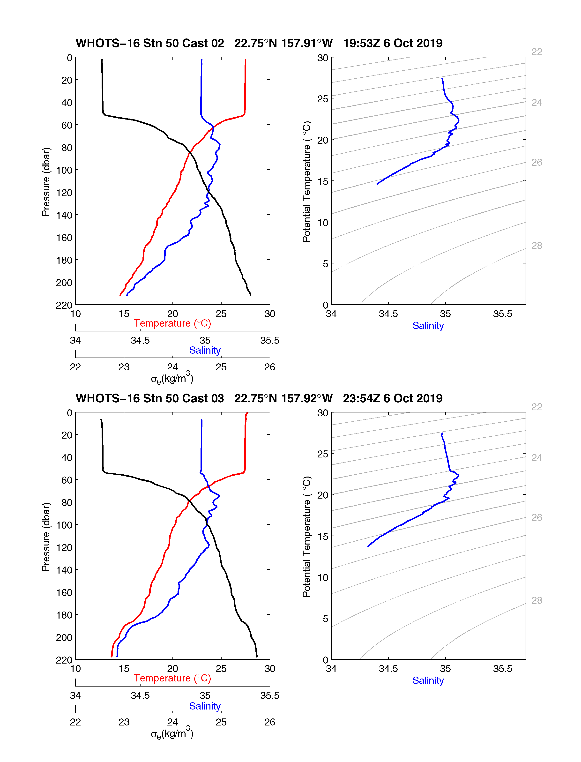
Fig. 6.2 [Upper panels] Same as in Fig. 6.1, but for station 50, cast 2. [Lower panels] Same as Fig. 6.1, but for station 50, cast 3.
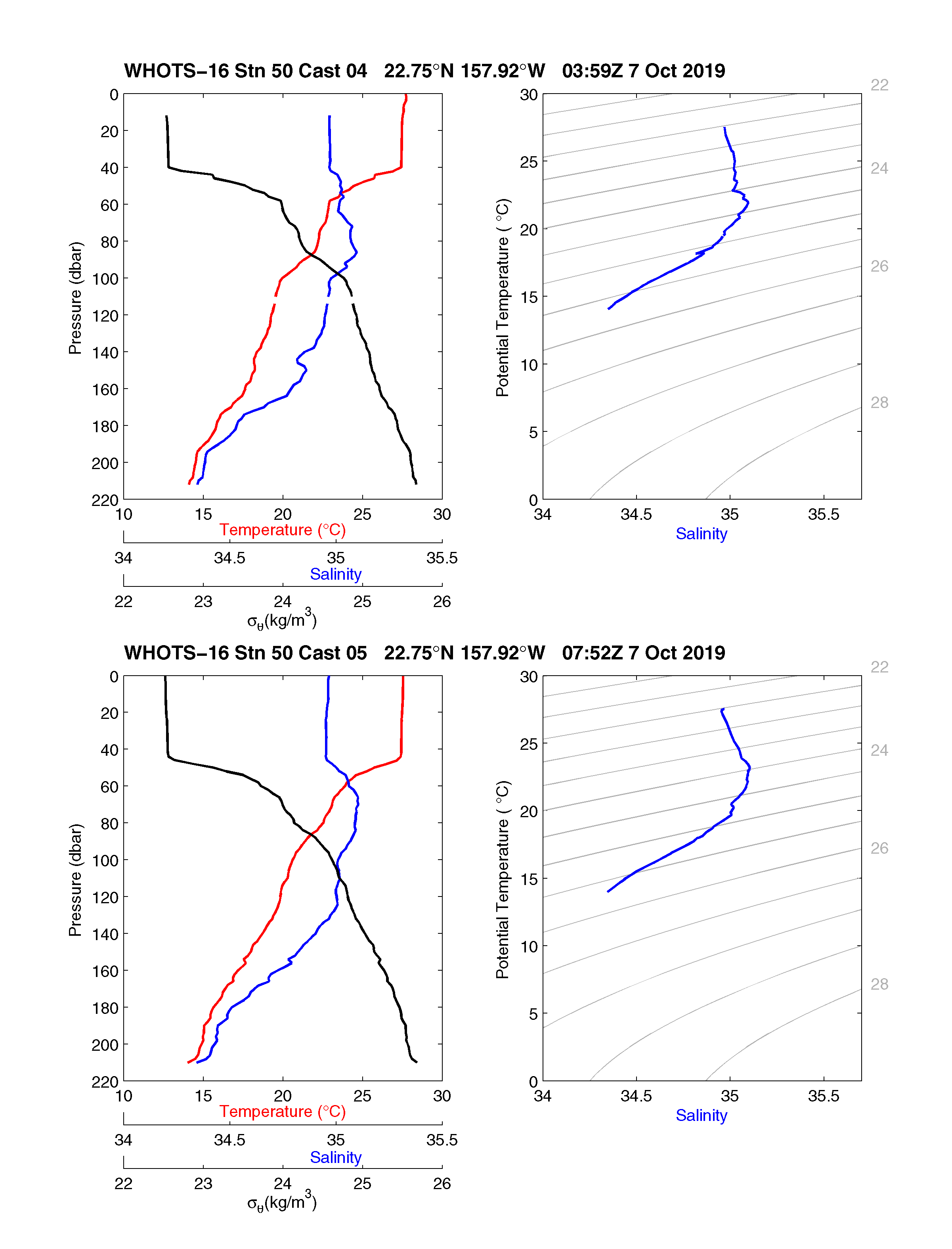
Fig. 6.3 [Upper panels] Same as in Fig. 6.1, but for station 50, cast 4. [Lower panels] Same as in Fig. 6.1, but for station 50 cast 5.
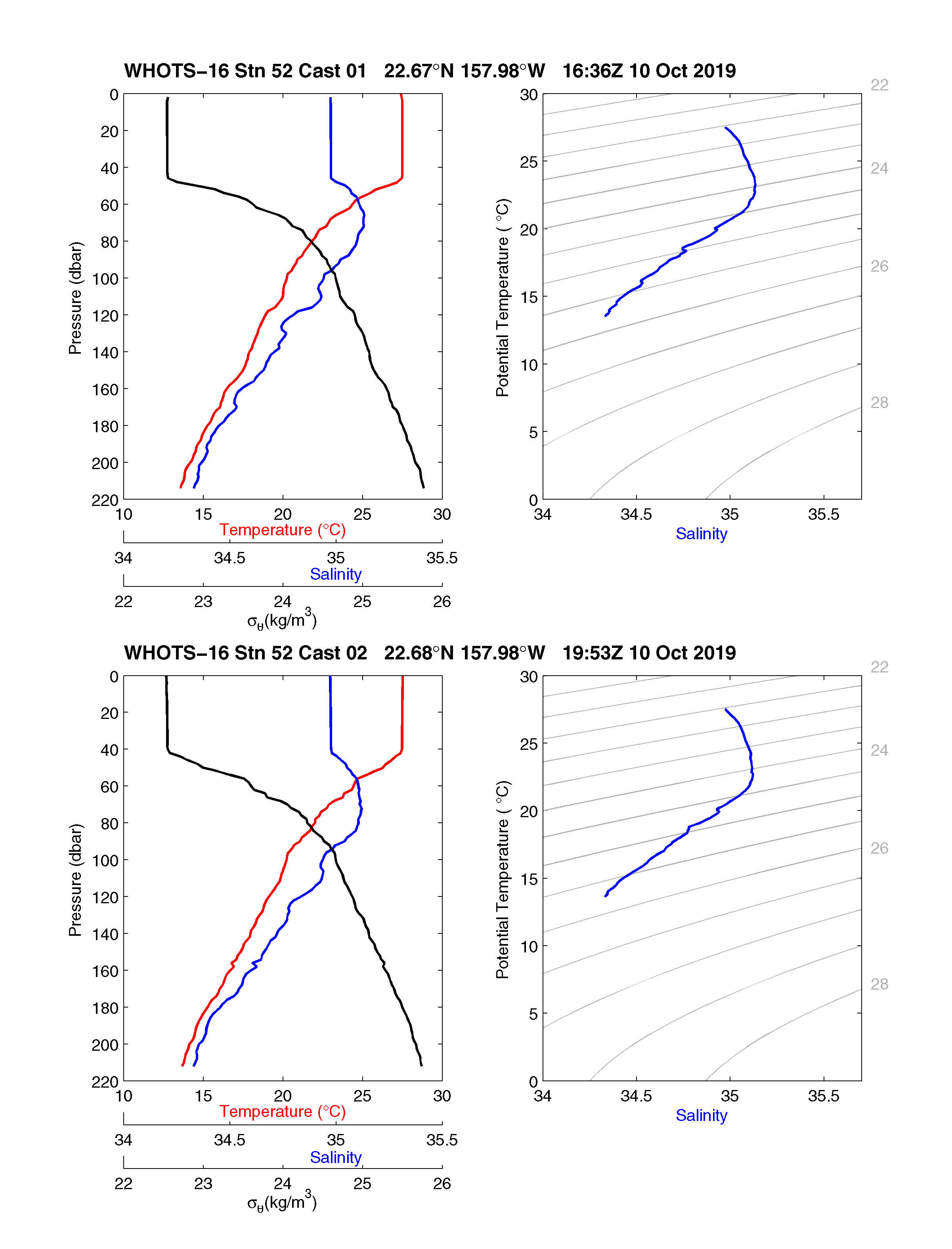
Fig. 6.4 [Upper panels] Same as in Fig. 6.1, but for station 52, cast 1. [Lower panels] Same as in Fig. 6.1, but for station 52, cast 2.
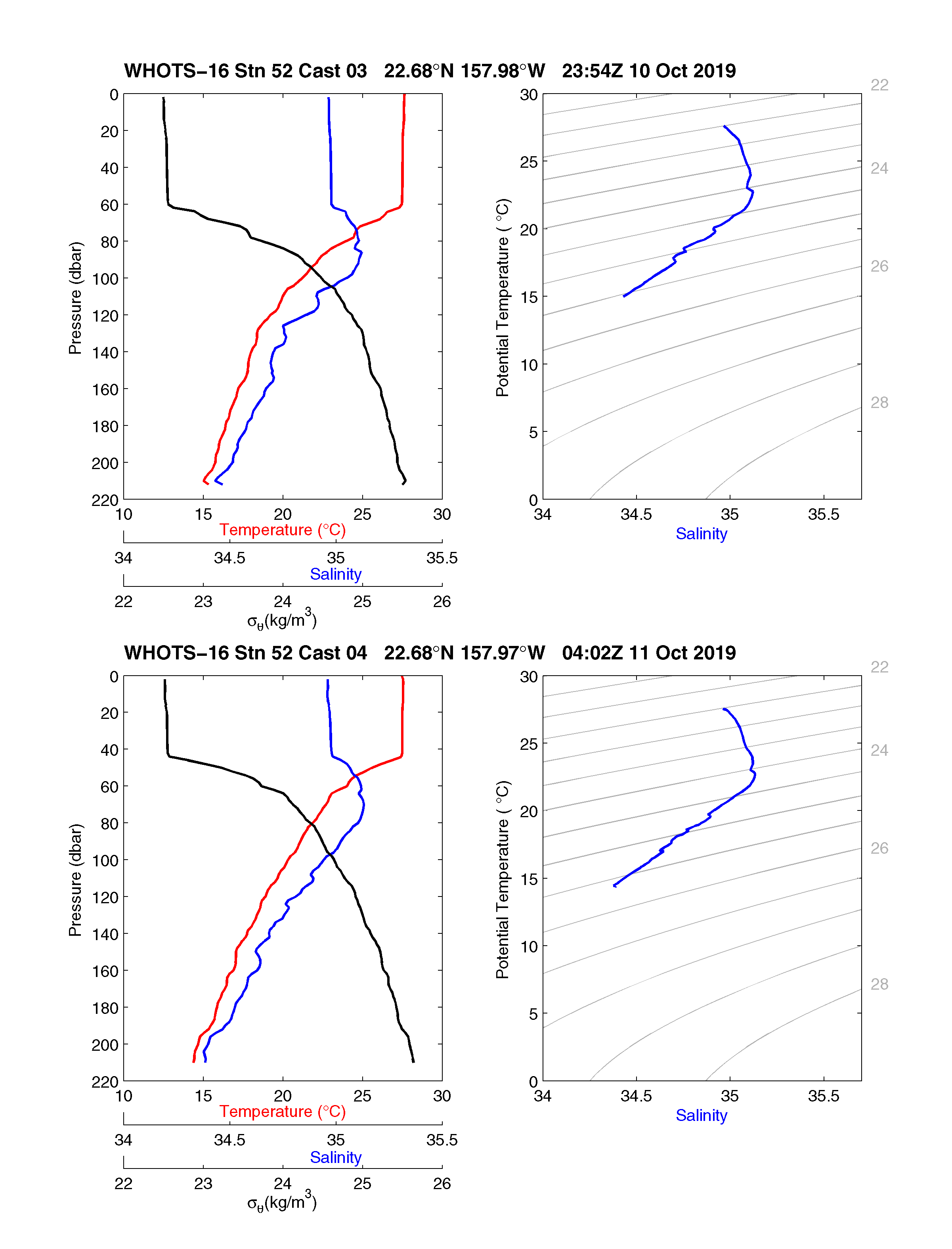
Fig. 6.5 Upper panels] Same as in Fig. 6.1, but for station 52, cast 3.[Lower panels] Same as in Fig. 6.1, but for station 52, cast 4.
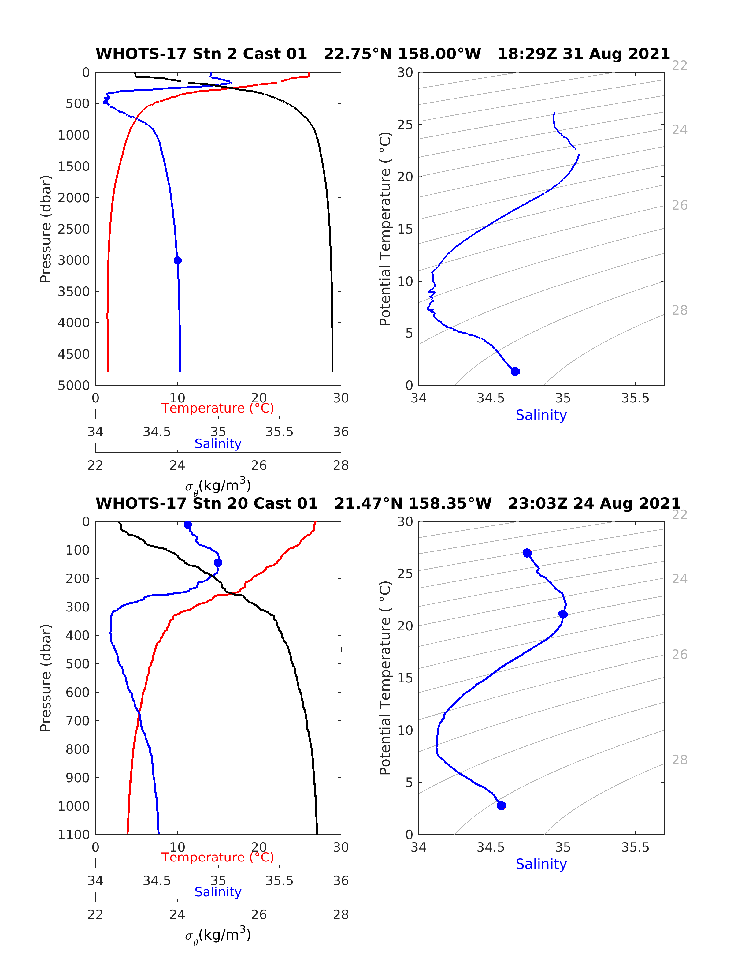
Fig. 6.6 [Upper left panel] Profiles of CTD temperature, salinity, and potential density (\(\sigma\theta\)) as a function of pressure, including discrete bottle salinity samples (when available) for station 2 cast 1 during the WHOTS-17 cruise. [Upper right panel] Profiles of CTD salinity as a function of potential temperature, including discrete bottle salinity samples (when available) for station 2 cast 1 during the WHOTS-17 cruise. [Lower left panel] Same as in the upper left panel, but for station 20 cast 1. [Lower right panel] Same as in the upper right panel, but station 20 cast 1.
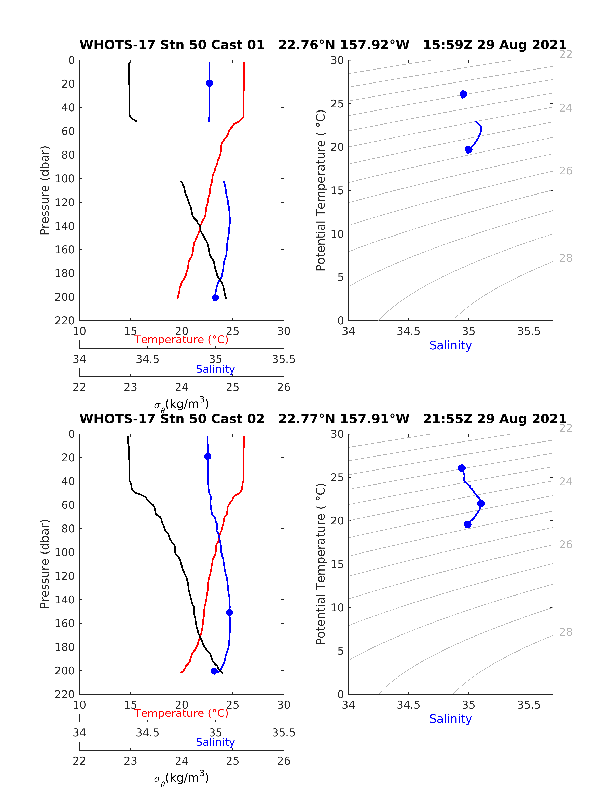
Fig. 6.7 Upper panels] Same as in Fig. 6.6, but for station 50, cast 1.[Lower panels] Same as in Fig. 6.6, but for station 50, cast 2.
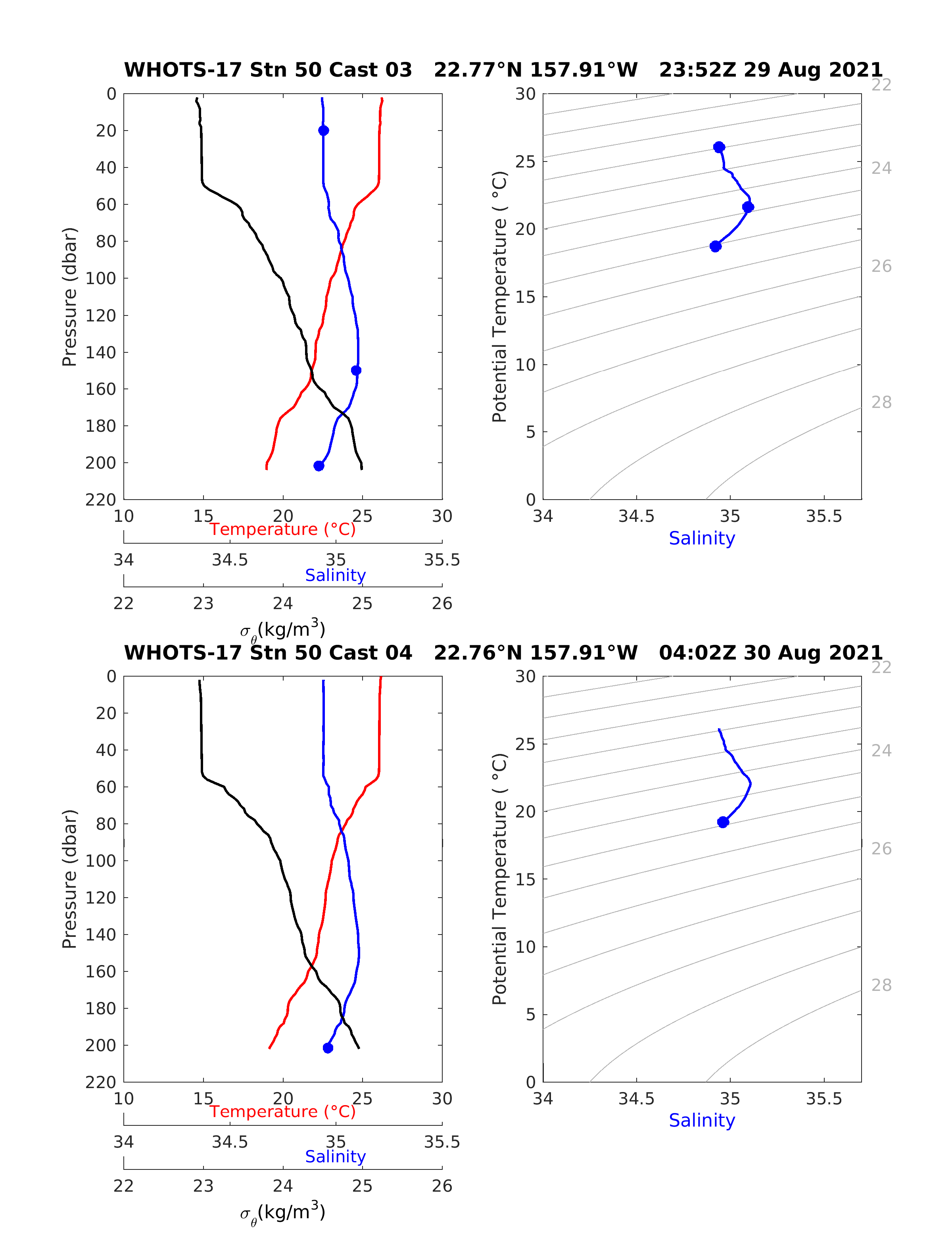
Fig. 6.8 Upper panels] Same as in Fig. 6.6, but for station 50, cast 3.[Lower panels] Same as in Fig. 6.6, but for station 50, cast 4.
6.2. Thermosalinograph Data
Underway measurements of near-surface temperature and salinity from the
thermosalinograph (TSG) system onboard the R/V Oscar Sette cruise are presented
in Fig. 6.11 and navigational data is shown in
Fig. 6.12 for the WHOTS-16 cruise. The WHOTS-16 underway
seawater system that feeds the TSG failed on October 11, 2019, due to air
going into the plumbing, causing the pumps to stop working during
deteriorated weather conditions. TSG and navigational data during the
WHOTS-17 cruise, onboard the R/V Oscar Sette, are presented in {numref}
ac40thsl_final.png and Fig. 6.14, respectively. The
data between August 25 and 27, 2021 are particularly bad because it was
during transit back to Oahu to disembark a crew member with medical
problems, and the flow through the system was stopped during that time.
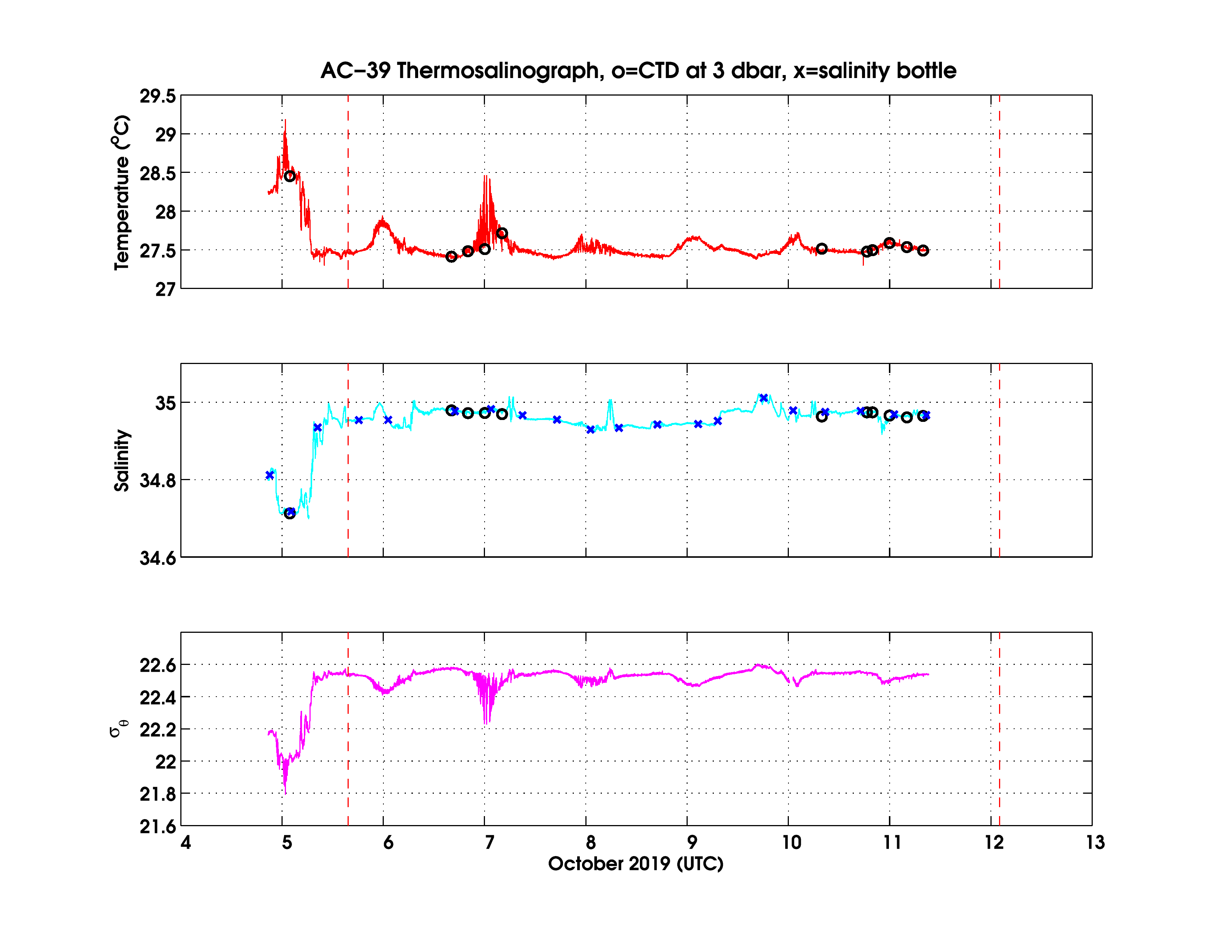
Fig. 6.11 Final processed temperature (upper panel), salinity (middle panel), and potential density (\(\sigma\theta\)) (lower panel) data from the continuous underway system onboard the R/V Hi’ialakai during the WHOTS-16 cruise. Temperature and salinity taken from 6-dbar CTD data (circles) and salinity bottle sample data (crosses) are superimposed. The dashed vertical red line indicates the period of occupation of Station ALOHA and the WHOTS site.
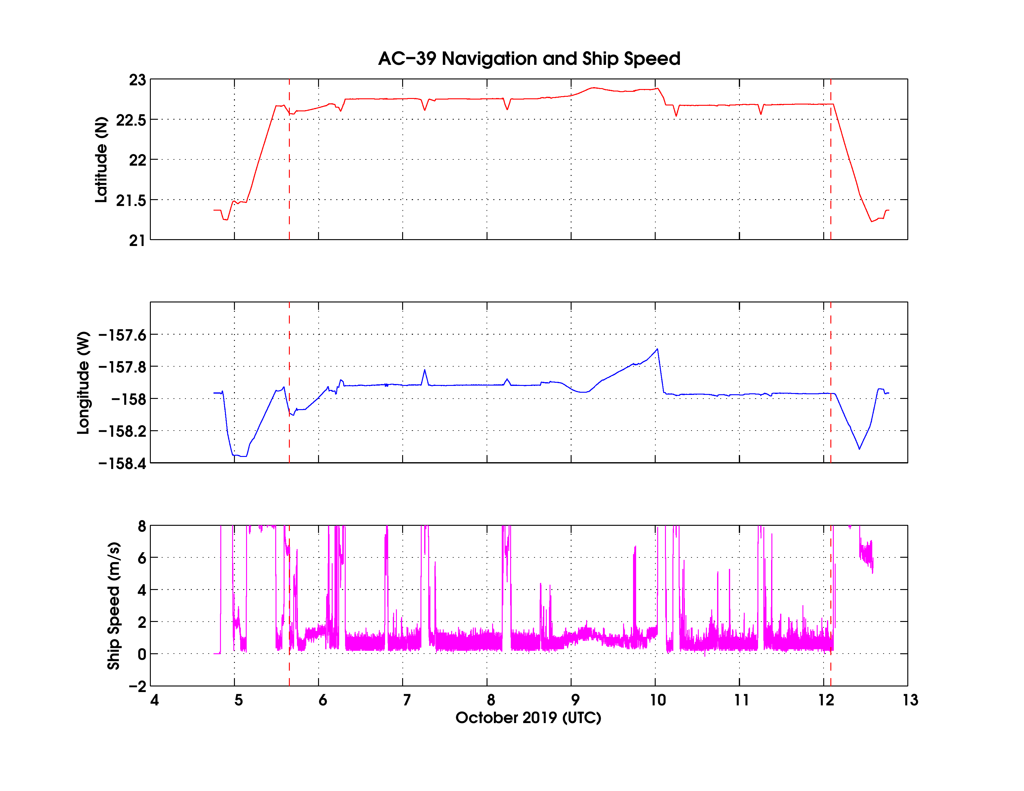
Fig. 6.12 Timeseries of latitude (upper panel), longitude (middle panel), and ship’s speed (lower panel) during the WHOTS-16 cruise.
Fig. 6.13 Final processed temperature (upper panel), salinity (middle panel), and potential density (\(\sigma\theta\)) (lower panel) data from the continuous underway system onboard the R/V Oscar Sette during the WHOTS-17 cruise. Temperature and salinity were taken from 6-dbar CTD data (circles), and salinity bottle sample data (crosses) are superimposed. The dashed vertical red line indicates the period of occupation of Station ALOHA and the WHOTS site.
Fig. 6.14 Timeseries of latitude (upper panel), longitude (middle panel), and ship’s speed (lower panel) during the WHOTS-17 cruise.
6.3. MicroCAT Data
The temperatures measured by MicroCATs during the mooring deployment for WHOTS-16 are presented in Fig. 6.15 through Fig. 6.20 for each of the depths where the instruments were located. The salinities are plotted in Fig. 6.21 through Fig. 6.26. The potential densities (\(\sigma\theta\)) are plotted in Fig. 6.27 through Fig. 6.32.
Contoured plots of temperature and salinity as a function of depth for the deployments WHOTS-1 through -16 are presented in Fig. 6.33, and contoured plots of potential density (\(\sigma\theta\)) as a function of depth are in Fig. 6.34, and of salinity as a function of \(\sigma\theta\) are in Fig. 6.35.
The potential temperature (\theta) and salinity measured by the deep MicroCATs during the mooring deployment are shown in Fig. 6.36. Also shown in the plot are the \theta and salinity data obtained with a MicroCAT (SBE-37) installed in the ALOHA Cabled Observatory, about six nautical miles north from the WHOTS-16 anchor. The instrument is located 2 m above the bottom.
Fig. 6.15 Temperatures from MicroCATs during WHOTS-16 deployment at 1.5, 7, 15, and 25 m.
Fig. 6.21 Salinities from MicroCATs during WHOTS-16 deployment at 1.5, 7, 15, and 25 m
Fig. 6.27 Potential densities (\(\sigma\theta\)) from MicroCATs during WHOTS-16 deployment at 1.5, 7, 15, and 25 m.
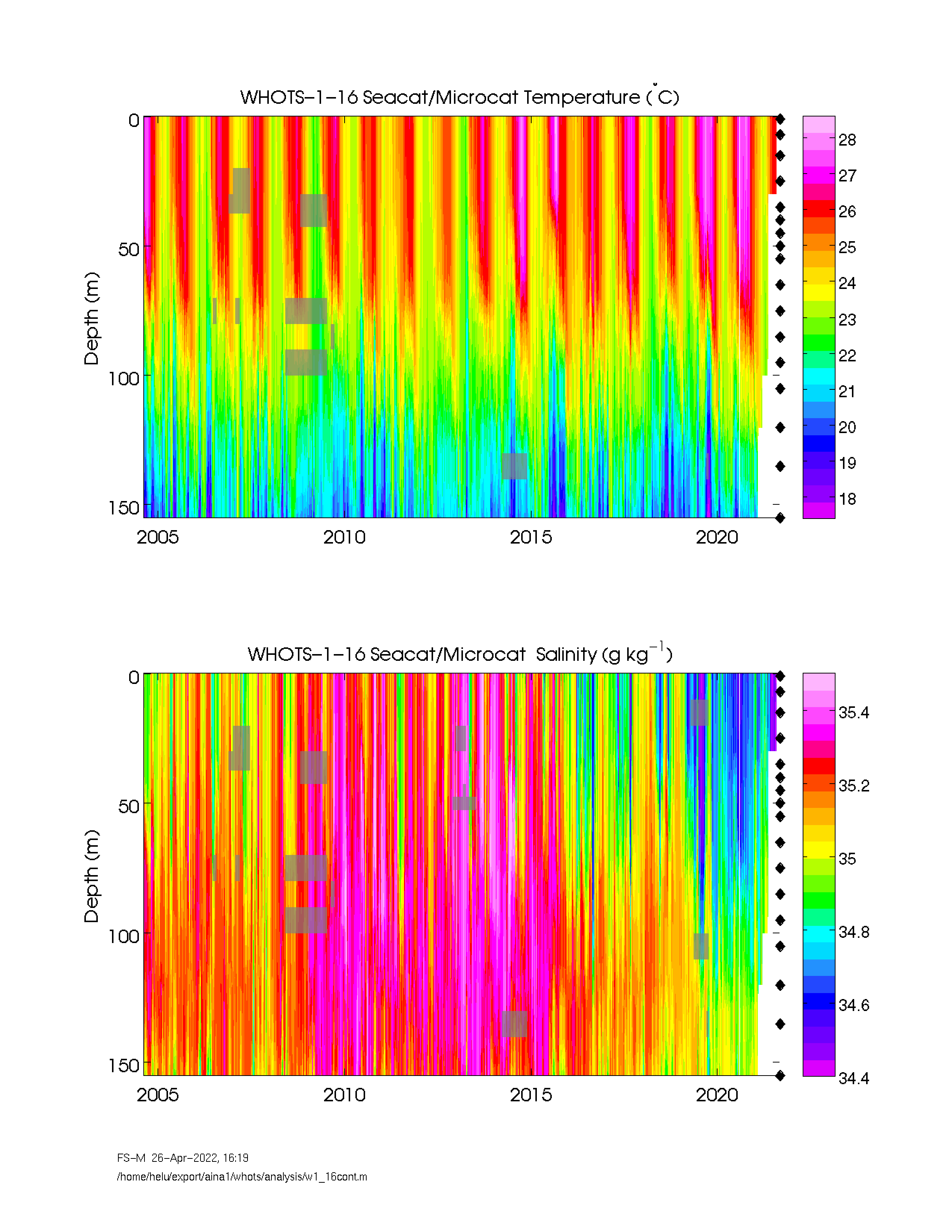
Fig. 6.33 Contour plots of temperature (upper panel) and salinity (lower panel) versus depth from SeaCATs/MicroCATs during WHOTS-1 through WHOTS-16 deployments. The shaded areas indicate missing data. The diamonds along the right axis indicate the depths of the instrument.
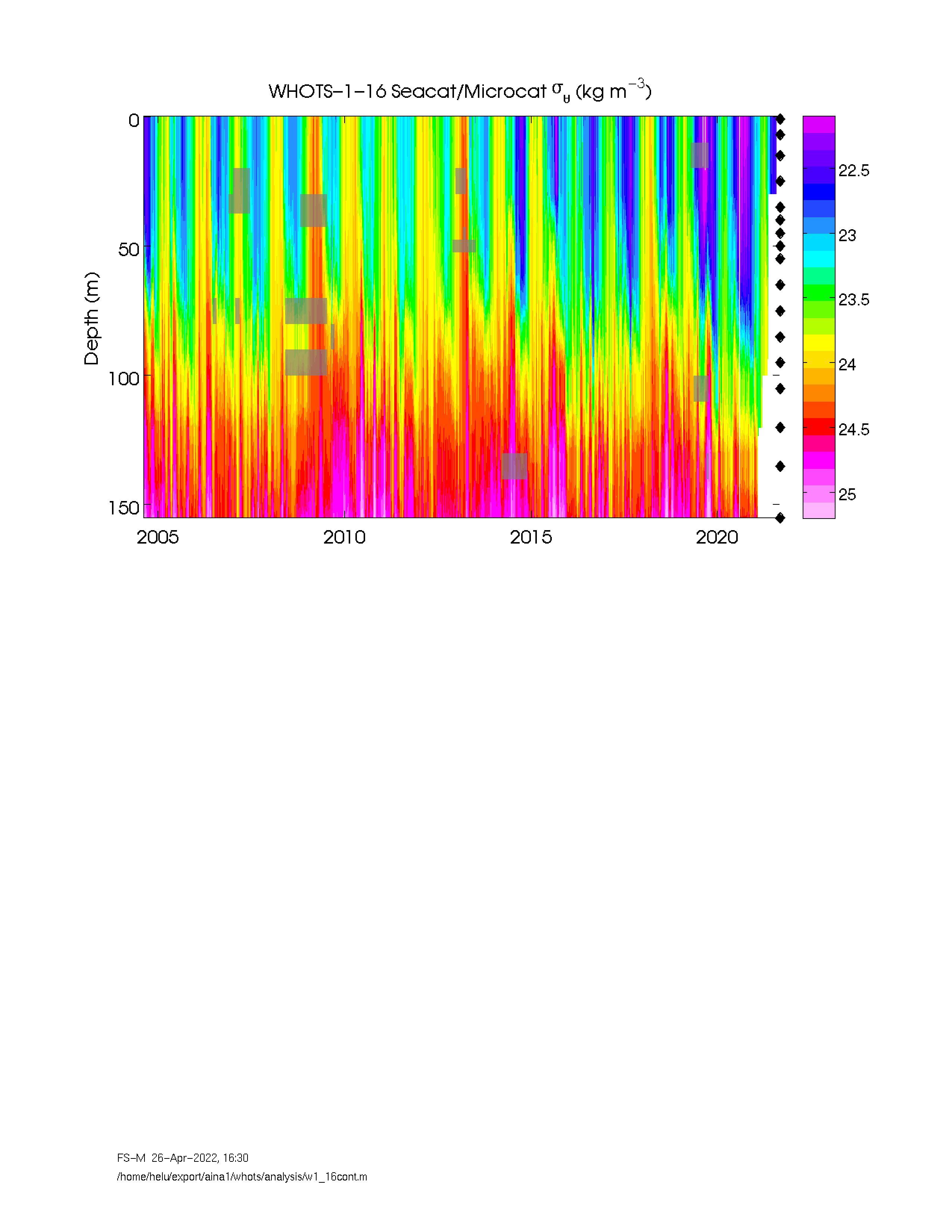
Fig. 6.34 Contour plots of potential density (\(\sigma\theta\)), versus depth from SeaCATs/MicroCATs during WHOTS-1 through WHOTS-16 deployments. The shaded areas indicate missing data. The diamonds along the right axis in the upper figure indicate the depths of the instrument.
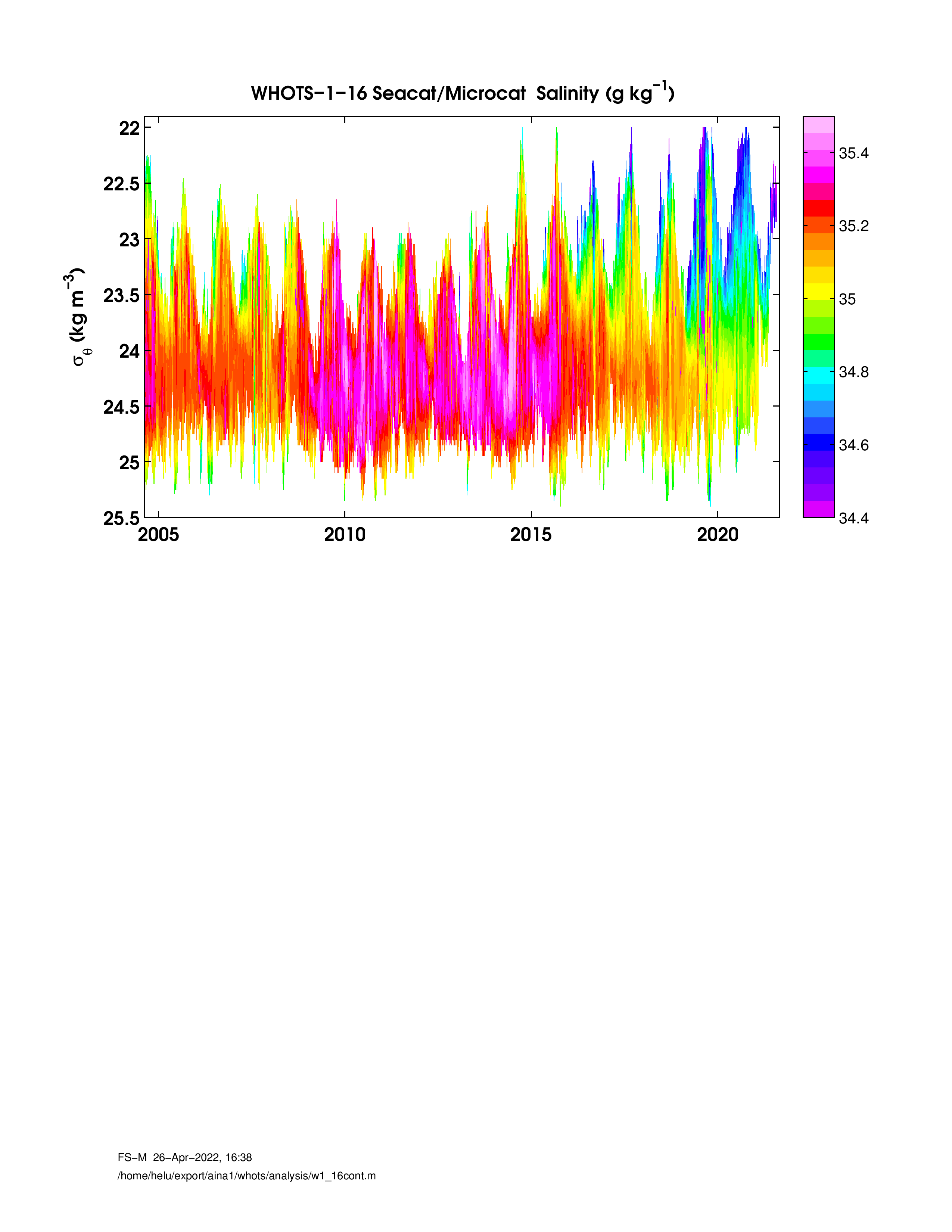
Fig. 6.35 Contour plots of salinity versus \(\sigma\theta\) from SeaCATs/MicroCATs during WHOTS-1 through WHOTS-16 deployments.
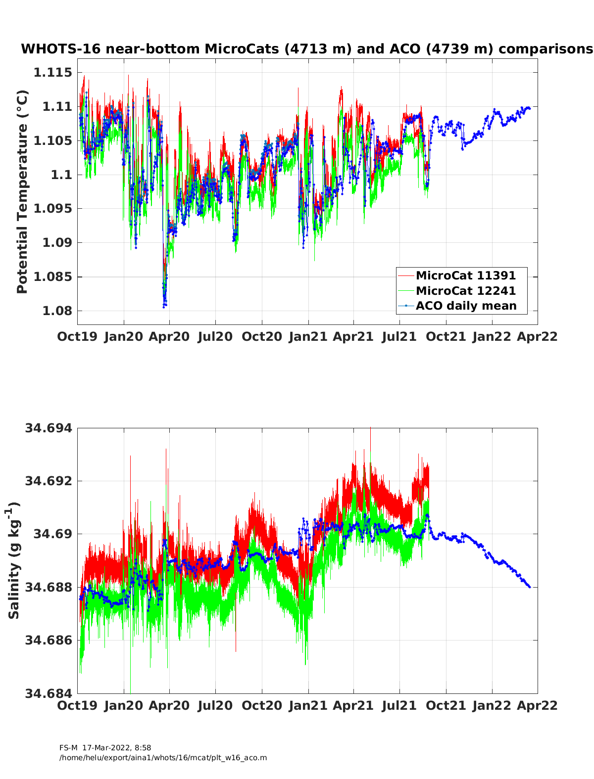
Fig. 6.36 Potential temperature (upper panel) and salinity (lower panel) time-series from the ALOHA Cabled Observatory (ACO) sensors and the WHOTS-16 MicroCATs 11391 and 12241.
6.4. Moored ADCP Data
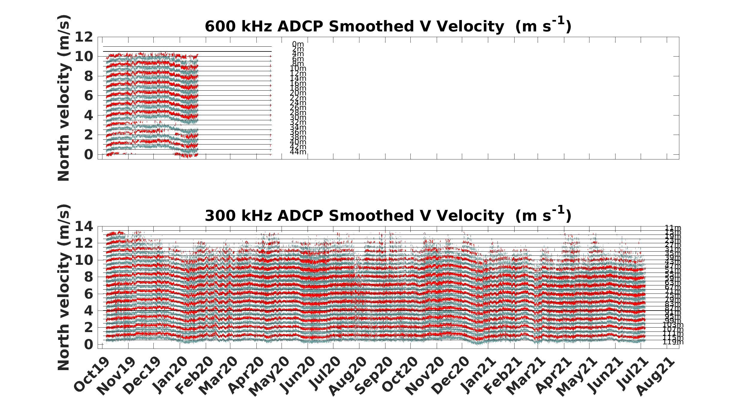
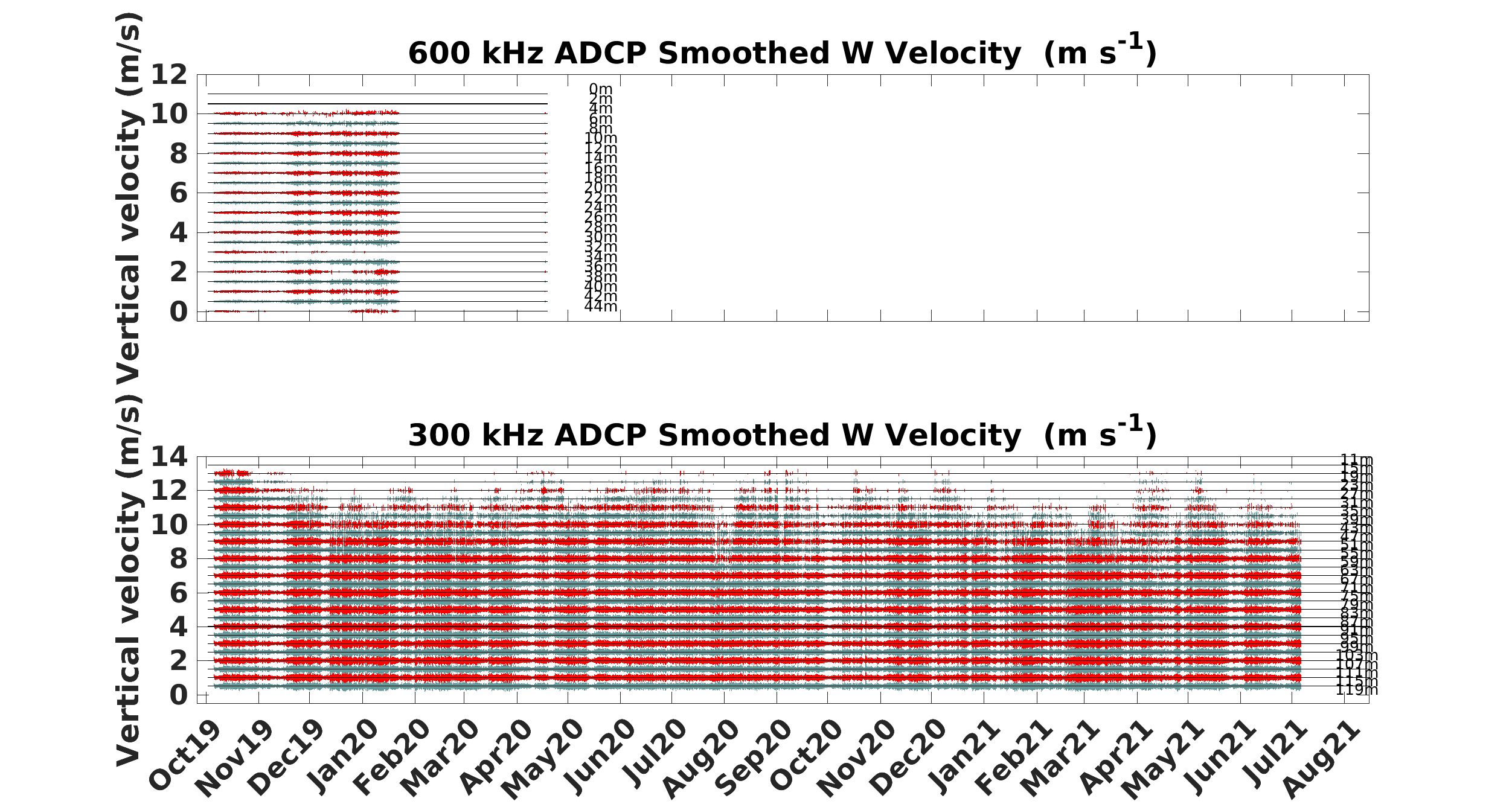
Contoured plots of smoothed horizontal (east and north component) and vertical velocity as a function of depth during the mooring deployments 1 through 16 are presented in Fig. 6.37 and Fig. 6.38. A staggered time-series of smoothed horizontal and vertical velocities are shown in Fig. 6.39 through Fig. 6.41. Smoothing was performed by applying a daily running mean to the data and then interpolating it on an hourly grid.
Contours of east and north velocity components from the Ship Oscar Sette Ocean Surveyor broadband 75 kHz shipboard ADCP, and the moored 300 kHz ADCP from the WHOTS-16 deployment as a function of time and depth, during the WHOTS-16 cruise, are shown in Fig. 6.42 and Fig. 6.43.
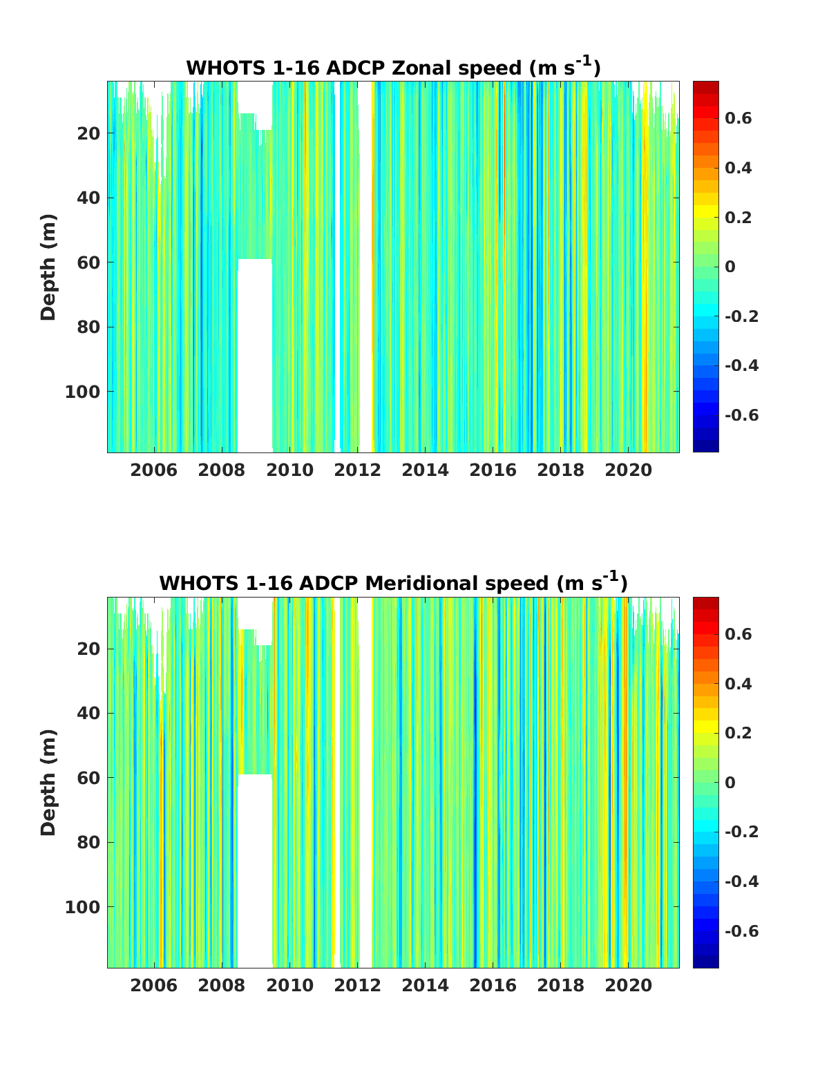
Fig. 6.37 Contour plot of east velocity component (\(m s^{-1}\)) versus depth and time from the moored ADCPs from the WHOTS-1 through -16 deployments (upper panel). Contour plot of north velocity component (\(m s^{-1}\)) (lower panel).
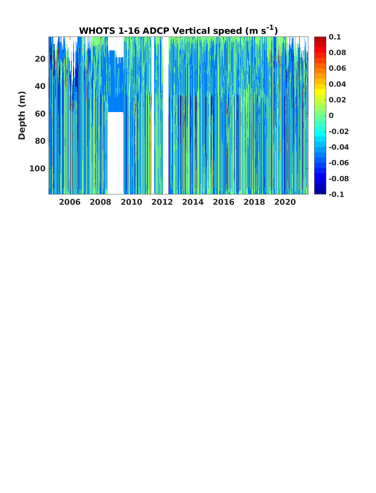
Fig. 6.38 Contour plot of vertical velocity component (\(m s^{-1}\)) versus depth and time from the moored ADCPs from the WHOTS-1 through -16 deployments.
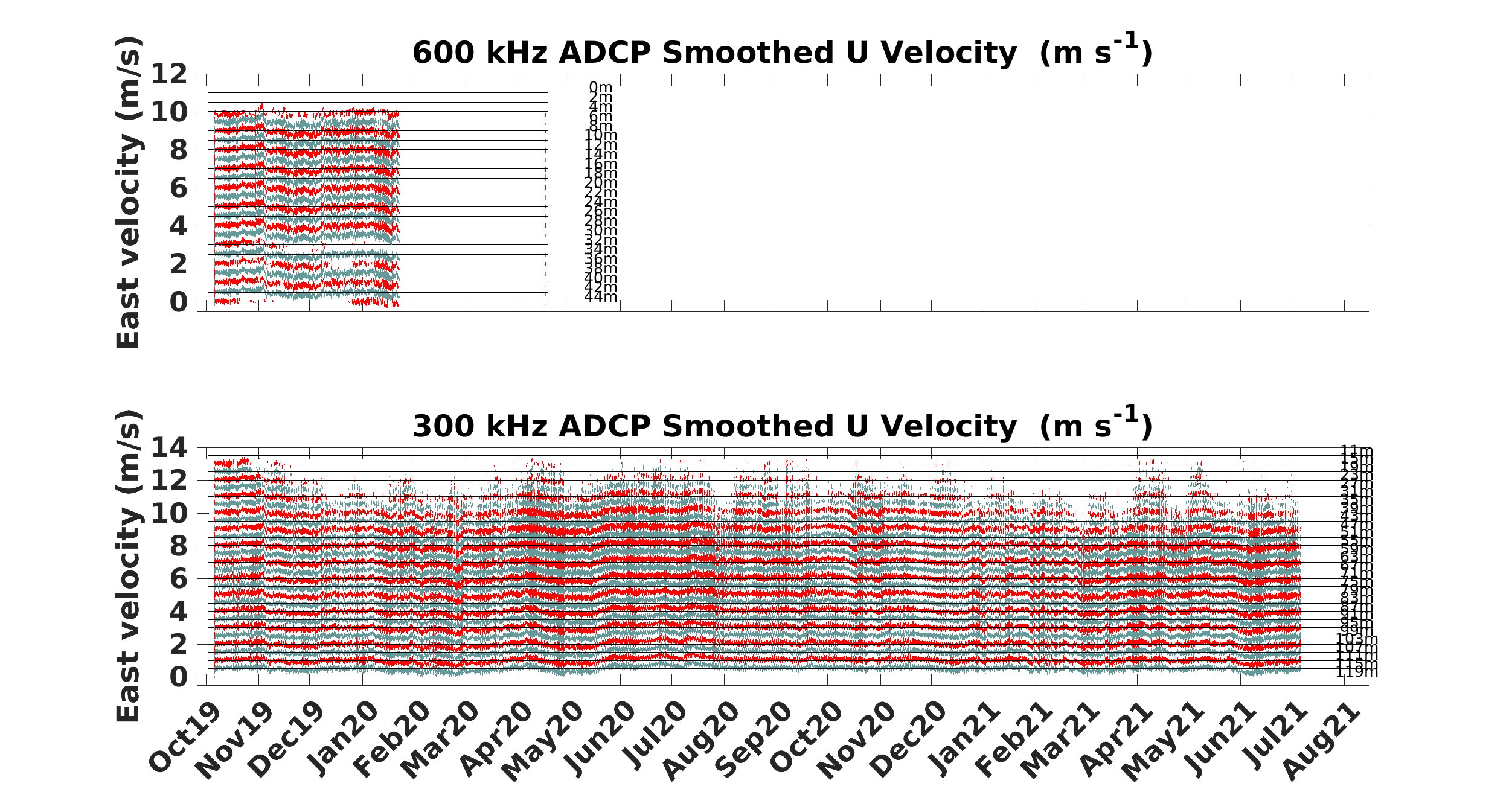
Fig. 6.39 Staggered time-series of east velocity component (\(m s^{-1}\)) for each bin of the 600 kHz (upper panel) and 300 kHz (lower panel) moored ADCPs during WHOTS-16. The time-series are offset upwards by 0.5 \(m s^{-1}\); each bin’s depth is on the right.
6.5. Moored and Shipboard ADCP comparisons
Contours of zonal and meridional current components from the Oscar Sette’s Ocean Surveyor broadband 75 kHz shipboard ADCP, and the moored 300 kHz ADCP from the WHOTS-16 deployment as a function of time and depth, during the WHOTS-16 cruise, are shown in Fig. 6.42. and Fig. 6.43. Similar comparisons during the WHOTS-17 cruise are in Fig. 6.44. and Fig. 6.45.
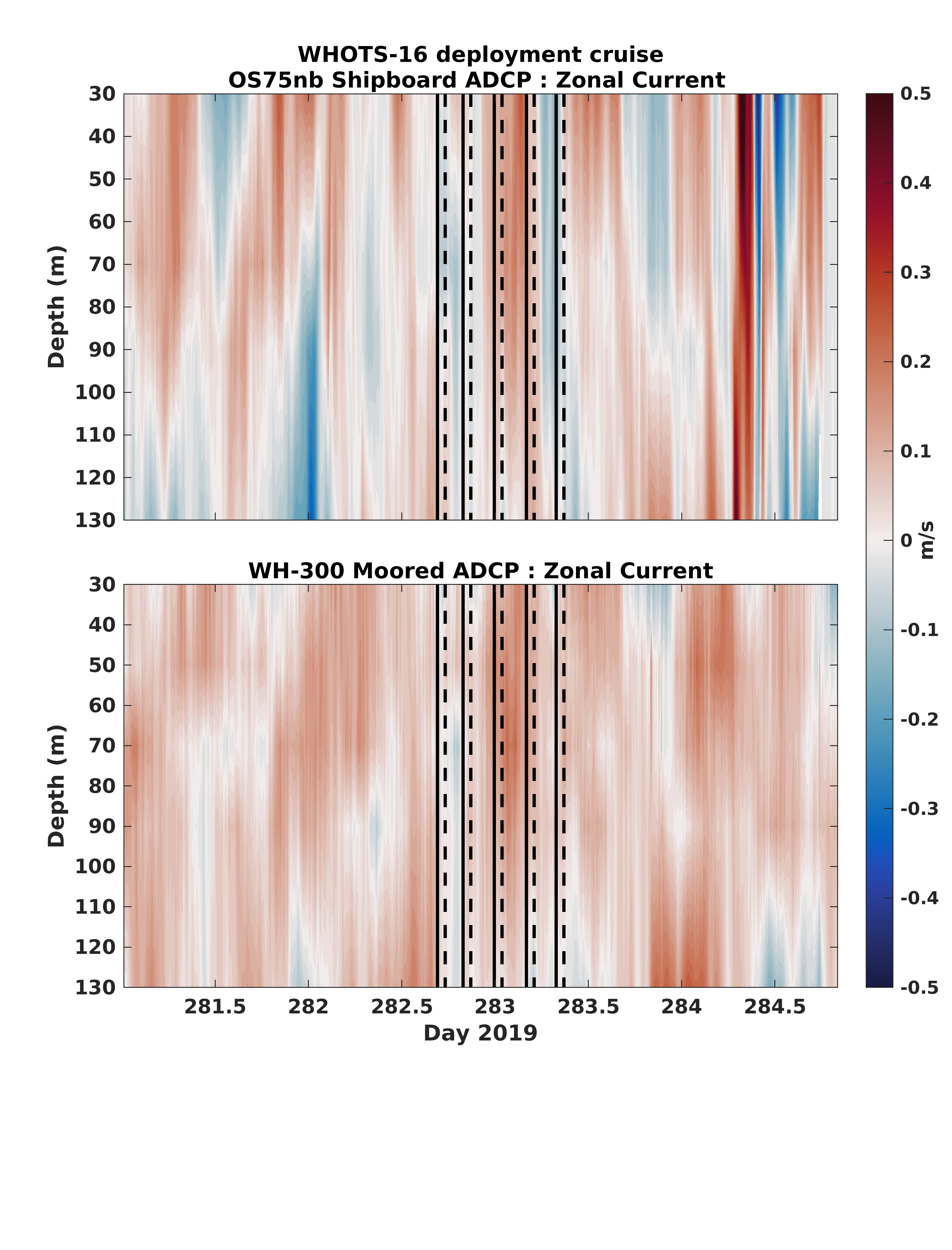
Fig. 6.42 The contour of zonal currents (\(m s^{-1}\)) from the Ship Oscar Sette Ocean Surveyor narrowband 75 kHz shipboard ADCP (upper panel), and the moored 300 kHz ADCP from the WHOTS-16 mooring (bottom panel) as a function of time and depth, during the WHOTS-16 cruise. Times when the CTD rosette was in the water are identified between solid and dashed black lines.
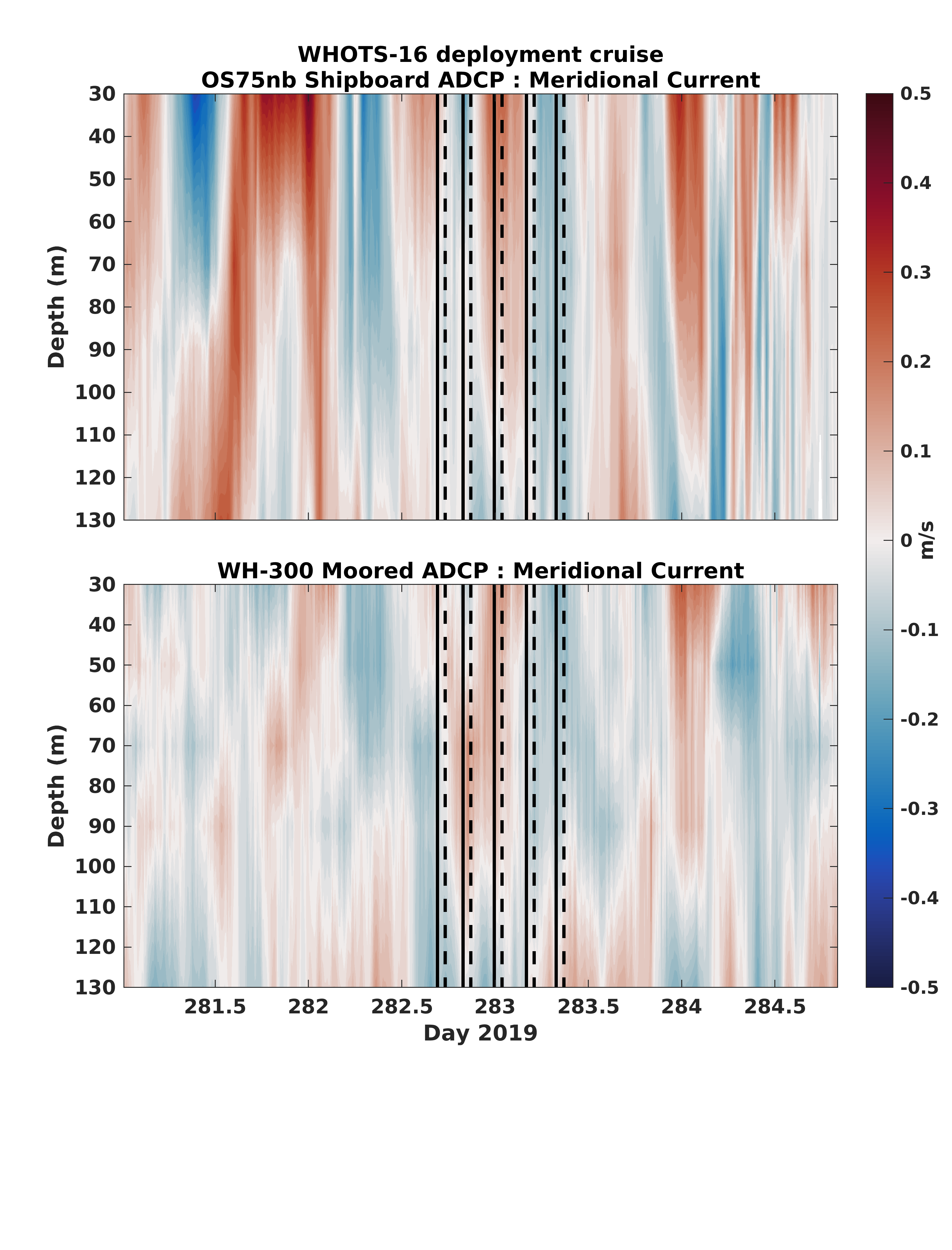
Fig. 6.43 The contour of meridional currents (\(m s^{-1}\)) from the Ship Oscar Sette Ocean Surveyor narrowband 75 kHz shipboard ADCP (upper panel), and the moored 300 kHz ADCP from the WHOTS-16 mooring (bottom panel) as a function of time and depth, during the WHOTS-16 cruise. Times when the CTD rosette was in the water are identified between solid and dashed black lines.
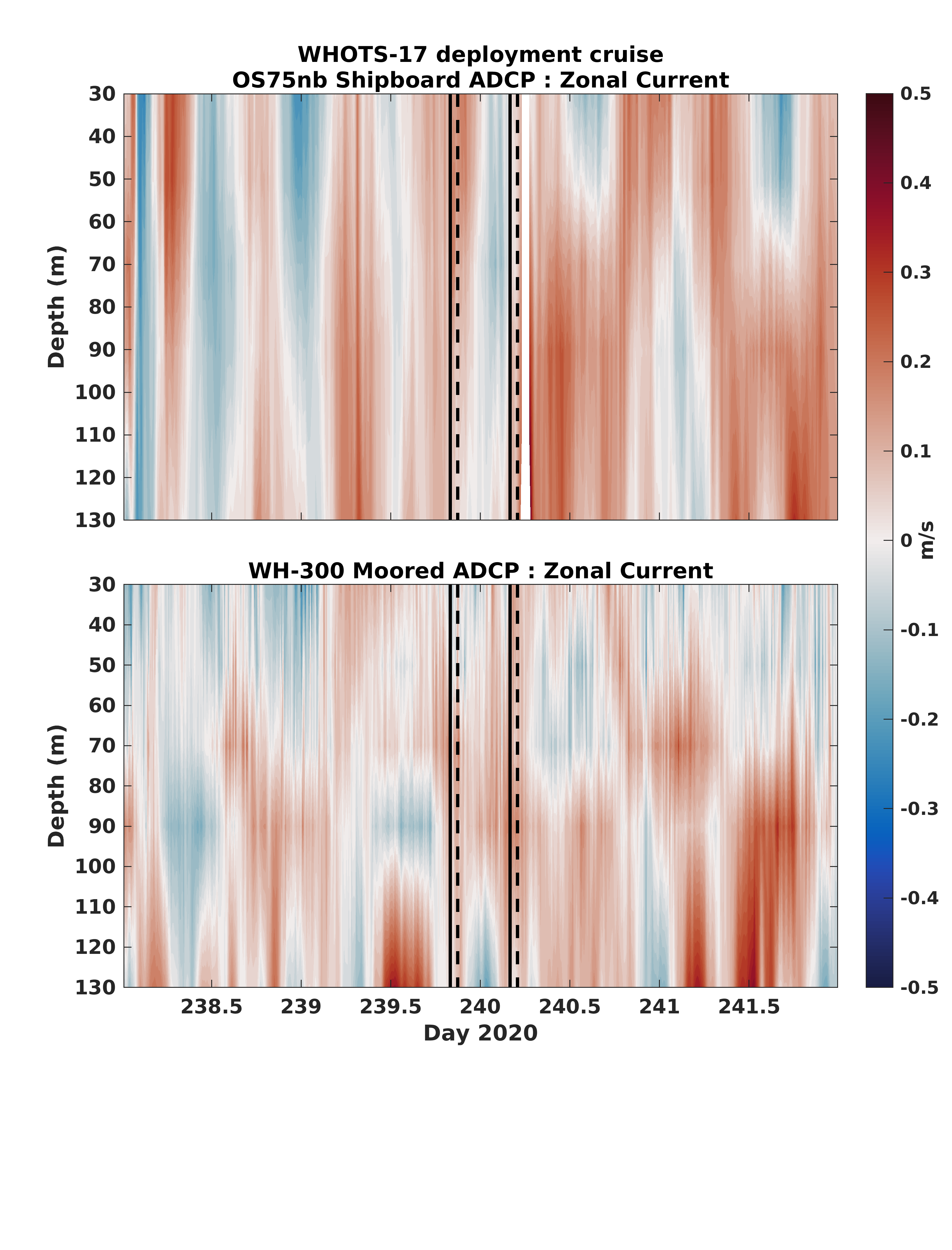
Fig. 6.44 The contour of zonal currents (\(m s^{-1}\)) from the Ship Oscar Sette Ocean Surveyor narrowband 75 kHz shipboard ADCP (upper panel), and the moored 300 kHz ADCP from the WHOTS-16 mooring (bottom panel) as a function of time and depth, during the WHOTS-17 cruise. Times when the CTD rosette was in the water are identified between solid and dashed black lines.
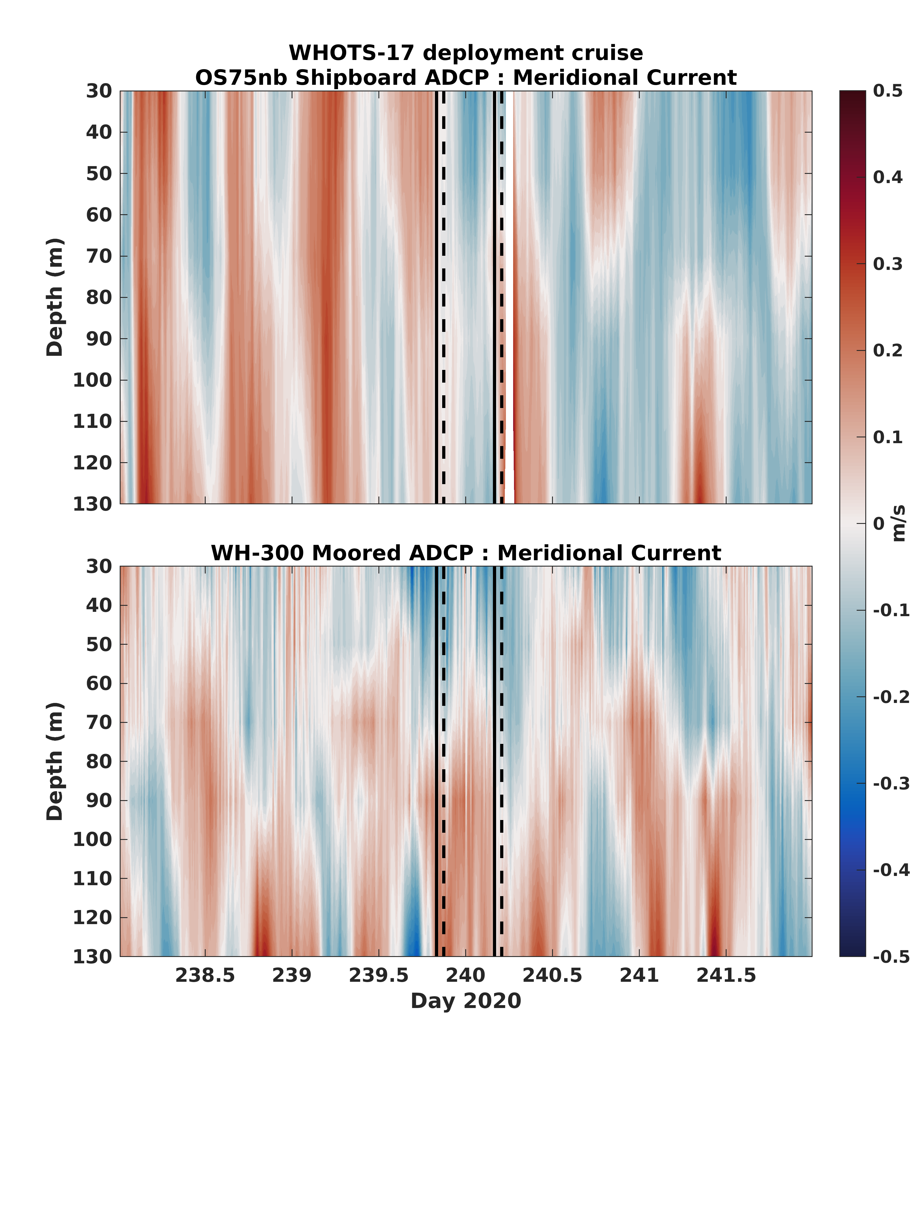
Fig. 6.45 Contours of meridional currents (\(m s^{-1}\)) from the Ship Oscar Sette Ocean Surveyor narrowband 75 kHz shipboard ADCP (upper panel), and the moored 300 kHz ADCP from the WHOTS-16 mooring (lower panel) as a function of time and depth, during the WHOTS-17 cruise. Times when the CTD/rosette was in the water are identified between the solid and dashed black lines.
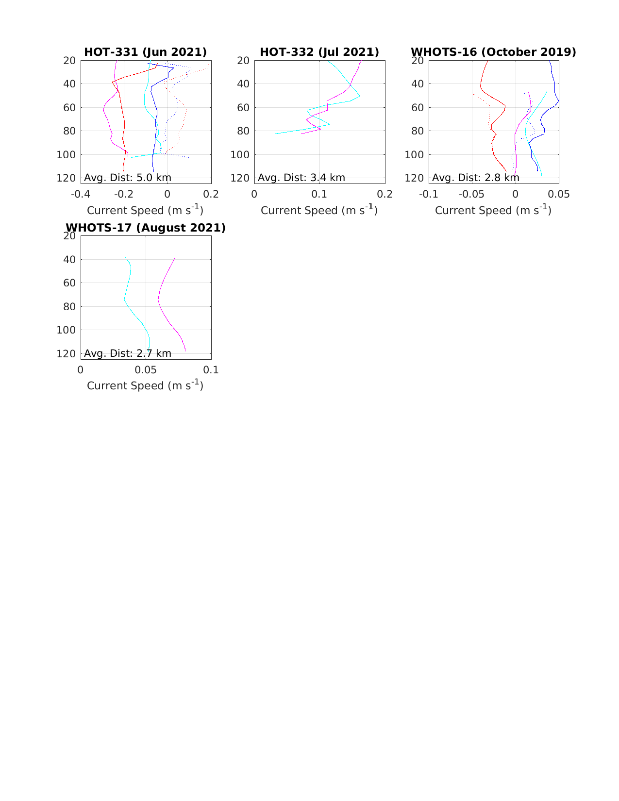
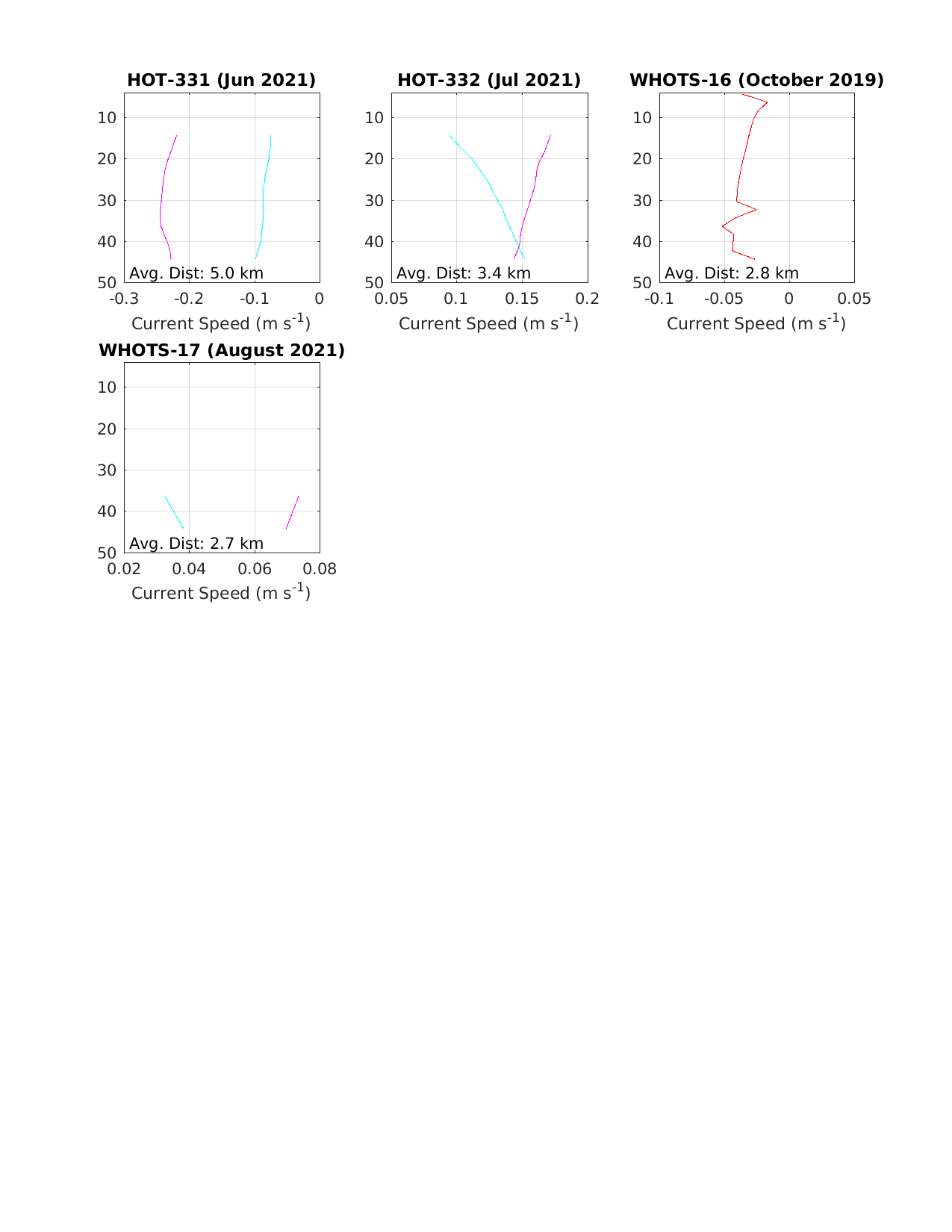
Comparisons between quality-controlled moored ADCPs during the WHOTS-16 deployment and available shipboard ADCP obtained during regular HOT cruises 316 to 332, and during the mooring deployment (WHOTS-16) and recovery (WHOTS-17) cruises are shown in Fig. 6.46 and Fig. 6.48 for the 300 kHz ADCP. Median and mean velocity profiles were computed when HOT CTD casts were being conducted near the WHOTS mooring specifically intended to calibrate moored instrumentation (see Conductivity Calibration). The HOT shipboard profiles were taken when the ship was stationary, within 1 km of the mooring, and within 4 hours before the start and 4 hours after the end of the CTD cast conducted near the WHOTS mooring.
HOT-316 was conducted on the R/V Oceanus and used data from TRDI Workhorse 300 kHz ADCP (wh300) with 2 m bin size, and averaging ensembles every 2 minutes; and from a TRDI Ocean Surveyor 75 kHz operating in broadband mode (os75nb) with 16 m bin size, with 5-minute ensemble interpolated to the profile resolution of the shipboard ADCP, and ensemble mean, and median profiles were obtained for each data set to compute differences and correlation coefficients between them.
HOT cruises conducted on the R/V Kilo Moana (HOT-317 to HOT-332) used data from a TRDI Workhorse 300 kHz ADCP (wh300) with 2 m bin size and averaging ensembles every 2 minutes; HOT-317 to HOT-319 and HOT-326 to HOT-332 used data from a TRDI Ocean Surveyor 38 kHz operating in broadband mode (os38bb) with 12 m bin size, with 5-minute ensemble interpolated to the profile resolution of the shipboard ADCP. HOT-317 to HOT-319 and HOT-326 to HOT-332 also used data from a TRDI Ocean Surveyor 38 kHz operating in narrowband mode (os38nb) with 24 m bin size, with 5-minute ensemble. HOT-324 only used data from the wh300 and os38nb (only three beams were working) instruments. HOT-326 also displayed issues with the os38 instrument.
Comparisons between the 300 kHz and the shipboard ADCP were available for HOT-316, HOT-318 to -325, HOT-327 to -329 (Fig. 6.46), and HOT-331 to -332 (Fig. 6.48); data from all others HOT cruises were excluded due to a lack of comparable data.
Comparisons between the moored 600 kHz and the shipboard ADCP were only available for HOT-316 and HOT-318 due to a mechanical issue with 600 kHz ADCP on January 21, 2020 (Fig. 6.47 and Fig. 6.49).
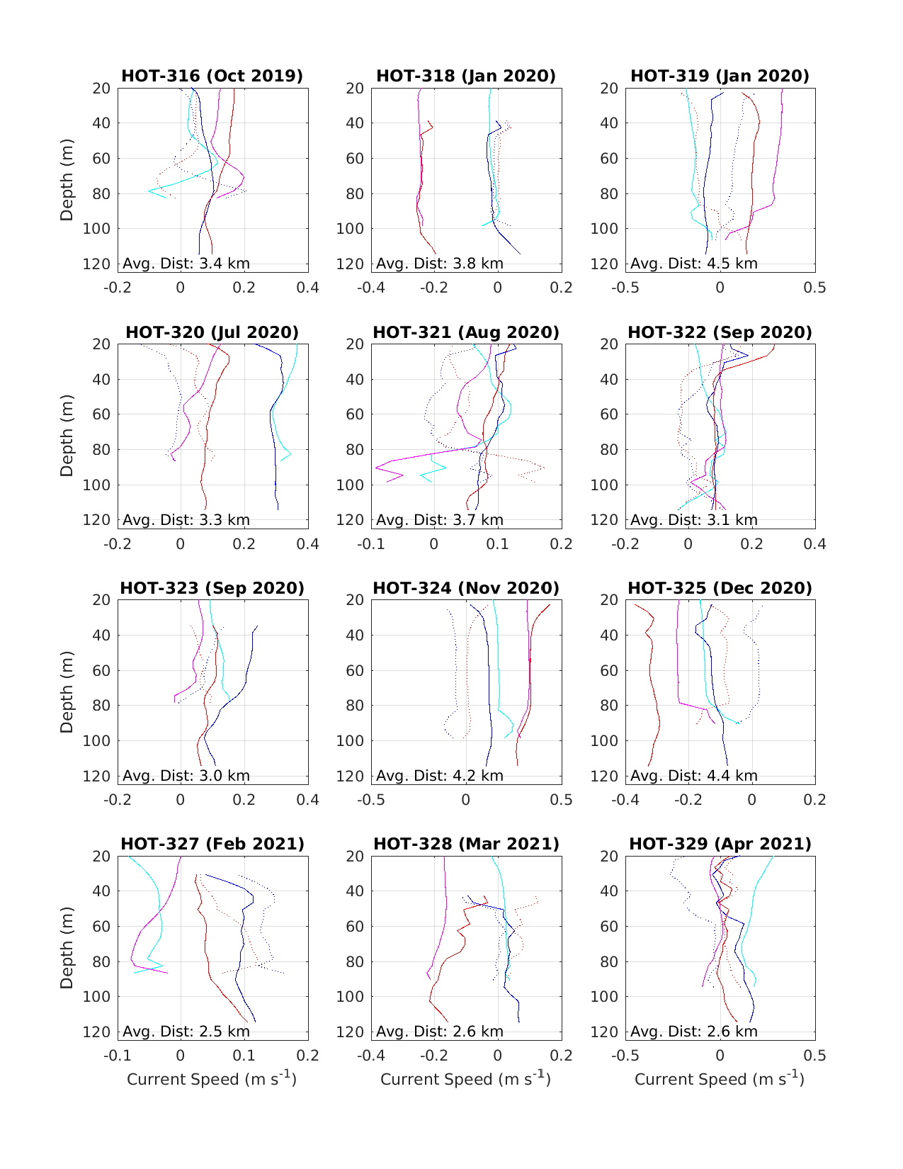
Fig. 6.46 Mean current profiles during shipboard ADCP (cyan: zonal, magenta: meridional) versus moored 300 kHz ADCP (blue: zonal, red: meridional) intercomparisons from HOT-316 through HOT-329. Moored minus shipboard ADCP differences shown in dotted lines (blue: zonal, red: meridional)
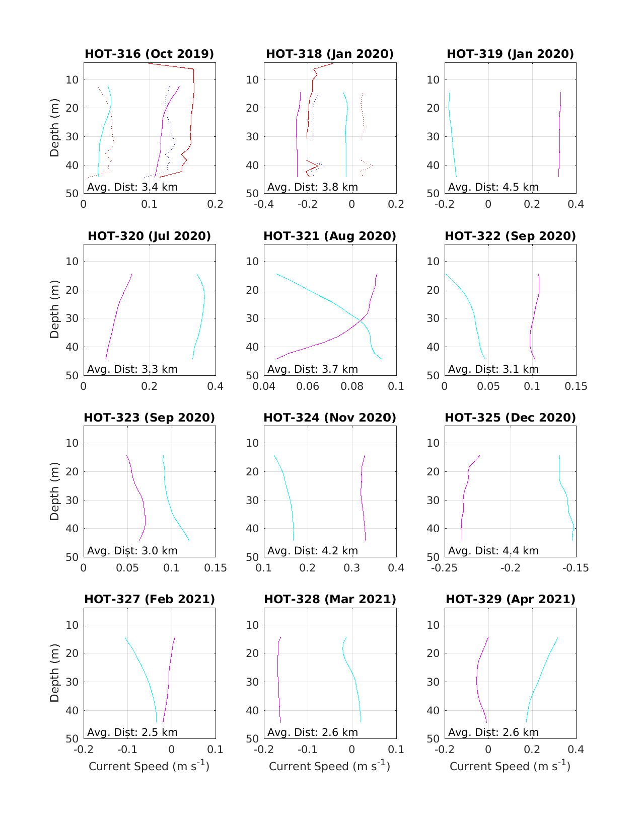
Fig. 6.47 Mean current profiles during shipboard ADCP (cyan: zonal, magenta: meridional) versus moored 600 kHz ADCP (blue: zonal, red: meridional) intercomparisons from HOT-316 through HOT-329. Moored minus shipboard ADCP differences shown in dotted lines (blue: zonal, red: meridional)
6.6. Next Generation Vector Measuring Current Meter Data (VMCM)
Time-series of daily mean horizontal velocity components for the VMCM current meters deployed during WHOTS-16 at 10 m and 30 m are presented in Fig. 6.50.
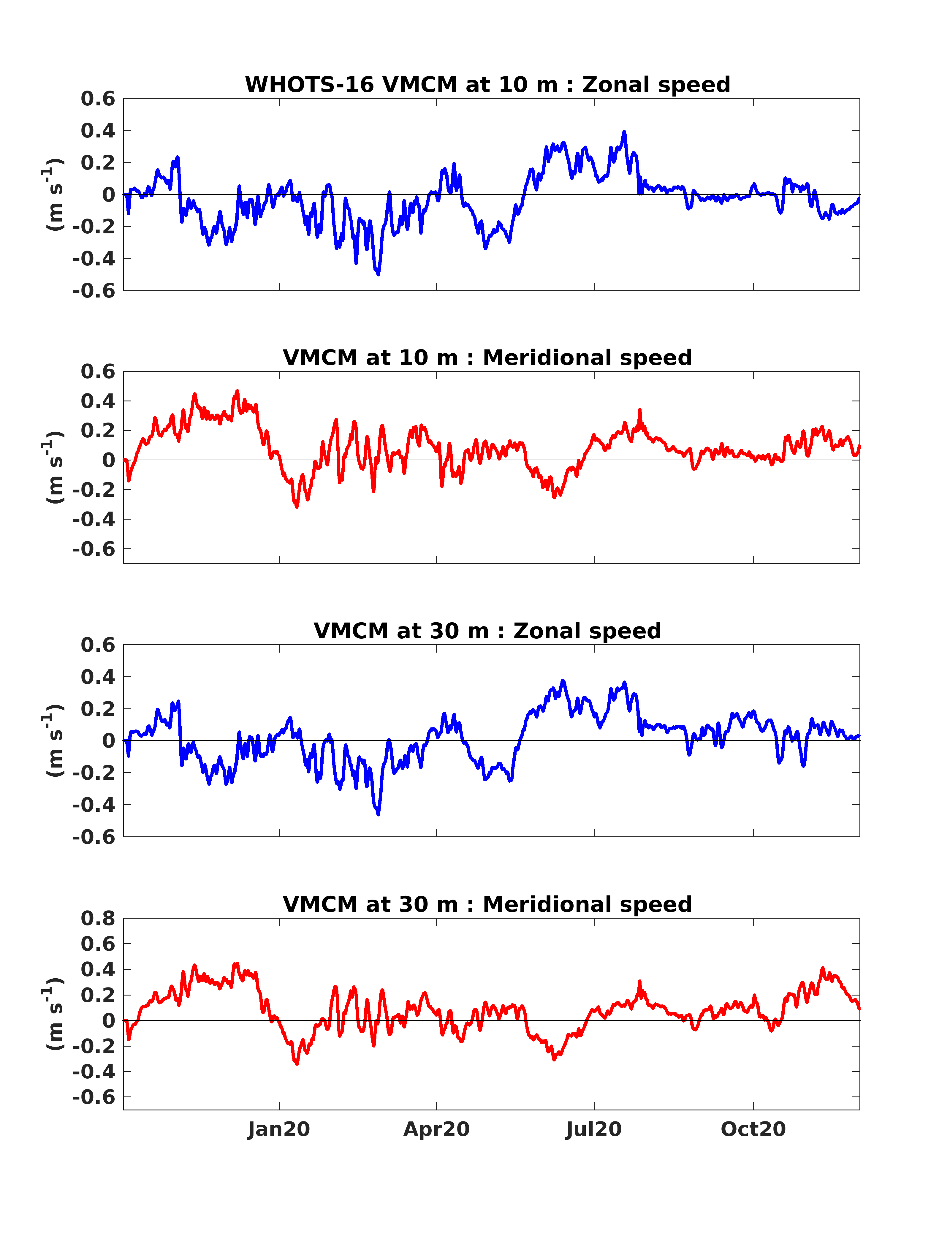
Fig. 6.50 Horizontal velocity data (\(m s^{-1}\)) during WHOTS-16 from the VMCMs at 10 m depth (first and second panel) and at 30 m depth (third and fourth panel)
6.7. GPS Data
Time-series of latitude and longitude of the WHOTS-16 buoy from GPS data are presented in Fig. 6.51, and spectra of the time-series are shown in Fig. 6.52.
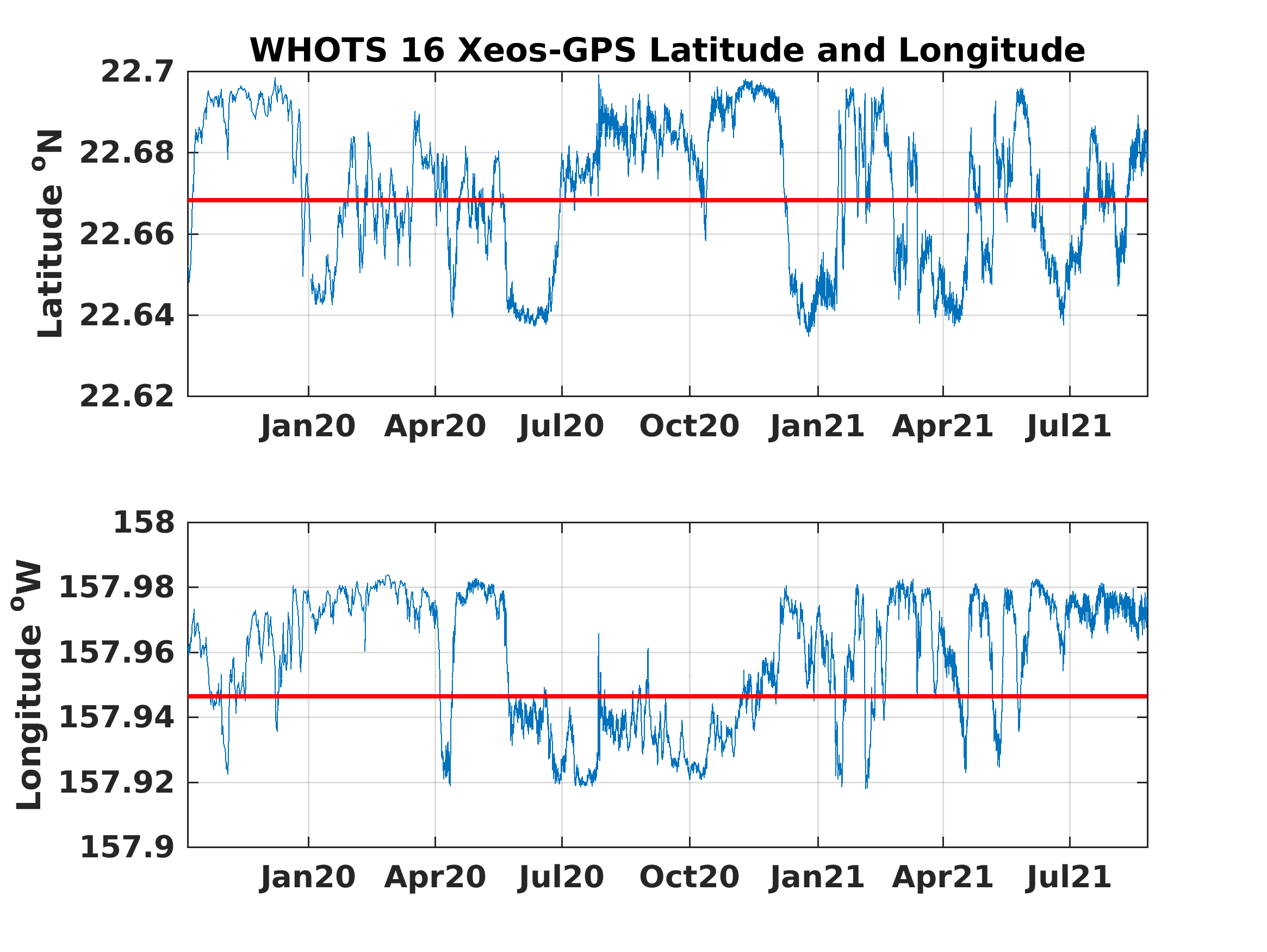
Fig. 6.51 GPS Latitude (upper panel) and longitude (lower panel) time series from the WHOTS-16 deployment.
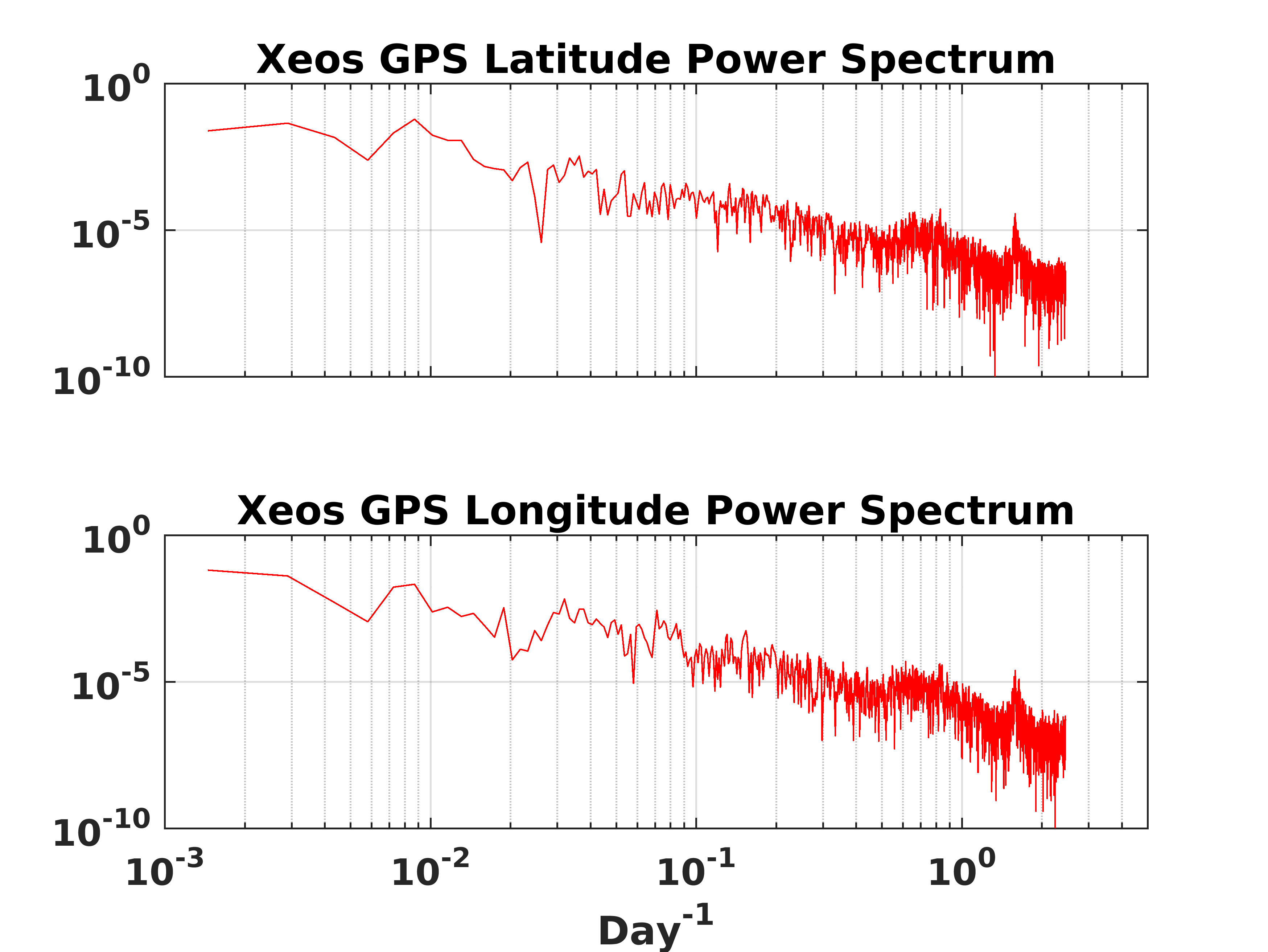
Fig. 6.52 The power spectrum of latitude (upper panel) and longitude (lower panel) for the WHOTS-16.
6.8. Mooring Motion
The position of the mooring with respect to its anchor was determined from the GPS positions. Additional information on the mooring motion was provided by the ADCP data of pitch, roll, and heading, shown in this section.
Fig. 6.53 shows the ADCP data of the instrument’s tilt (a combination of the pitch and roll), plotted against the buoy’s distance from its anchor (derived from GPS positions), for both WHOTS-16 ADCP’s. The plot’s red line is a quadratic fit to the median tilt calculated every 0.2 km distance bins. The figure shows that during both deployments, the ADCP tilt increased as the anchor’s distance increased. This tilting was caused by the mooring line’s deviation from its vertical position as the anchor pulled it. The tilting of the line also caused the rising of the instruments attached to the line. The 600 kHz ADCP failed in January 2021.
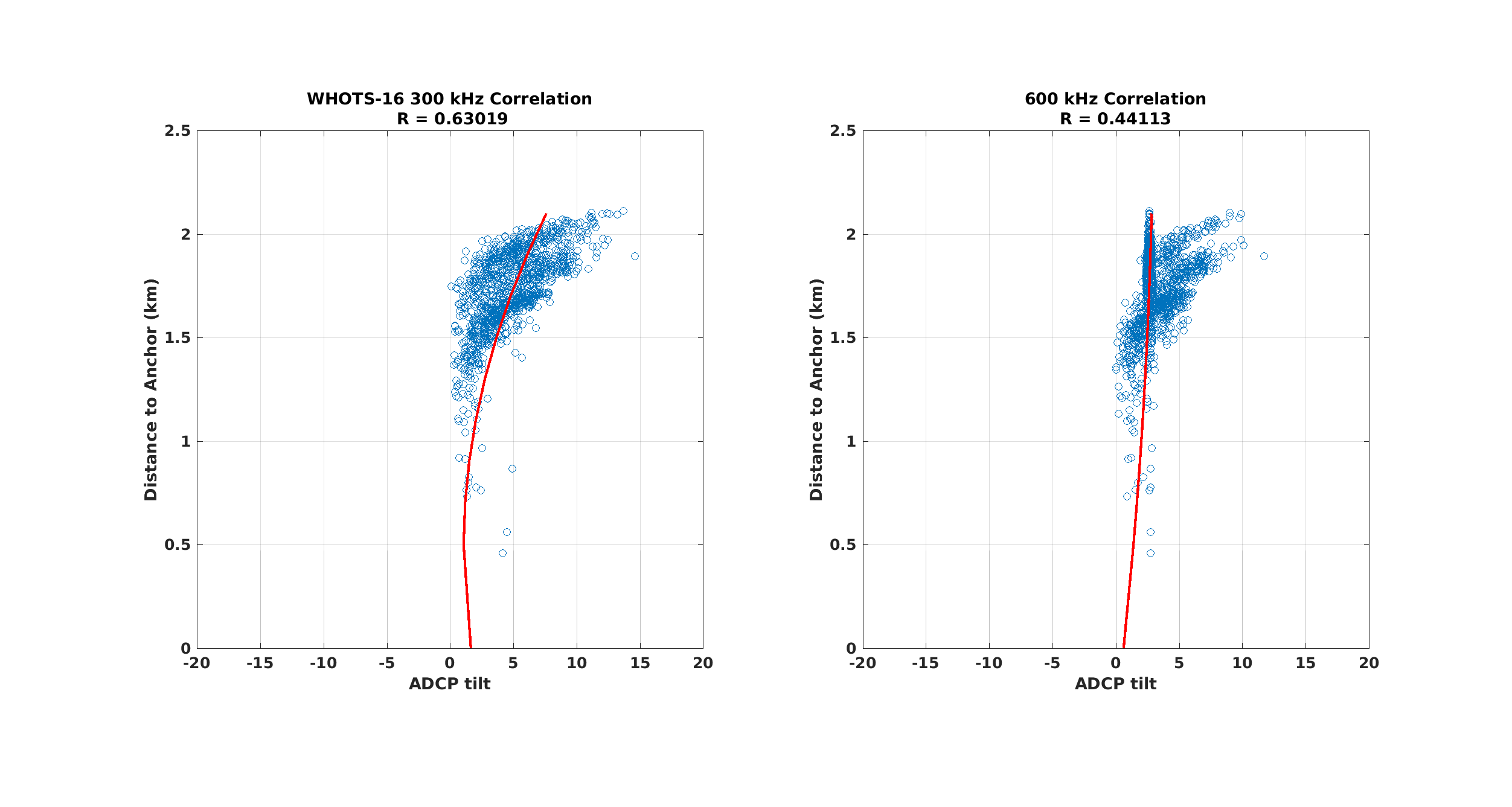
Fig. 6.53 Scatter plots of ADCP tilt and distance of the buoy to its anchor for the 300 kHz (left panel) and the 600 kHz ADCP deployments (right panel, blue circles). The red line is a quadratic fit to the median tilt calculated every 0.2 km distance bins.