Results
Contents
6. Results
During the WHOTS-18 cruise (WHOTS-18 mooring deployment, 24 July 2022), a high-pressure ridge far north of the Hawaiian Islands maintained a tight enough pressure gradient down across the region to produce moderate local trades, increasing by the end of the cruise. There was no measurable precipitation during the deployment or recovery times. Conditions during the WHOTS-18 deployment were favorable, with light ENE winds during the deployment. There were clear skies and no precipitation in the region, and small short-period wind waves.
Currents were nearly 1 kt to the west in the upper 200 m. This westward flow seemed to be associated with a high sea level north of Station ALOHA. A combination of internal semidiurnal and diurnal tides, along with near-inertial oscillations, were noticeable especially in vertical shear.
CTD casts conducted near the WHOTS-18 buoy (Station 52) after deployment (Fig. 6.3, Fig. 6.4, Fig. 6.5) displayed a subsurface salinity maximum between 60 and 80 dbar and a mixed layer 60 to 80 dbar deep.
During the WHOTS-19 cruise (WHOTS-18 mooring recovery, 19 June 2023), a high-pressure ridge far north of the Hawaiian Islands maintained a tight enough pressure gradient down across the region to produce moderate local trades, increasing by the end of the cruise. There was no measurable precipitation during the deployment or recovery times. Conditions during the WHOTS-19 deployment on June 16-17 were favorable. There were 15-16 kt winds from the east during the deployment and a westward current of nearly 0.5 kt near the surface. There were clear skies and no precipitation in the region, and there were small short-period wind waves.
Currents were predominantly to the northwest in the upper 200 m. This westward flow seemed to be associated with a high sea level north of Station ALOHA. A combination of internal semidiurnal and diurnal tides, along with near-inertial oscillations, were noticeable, especially in vertical shear.
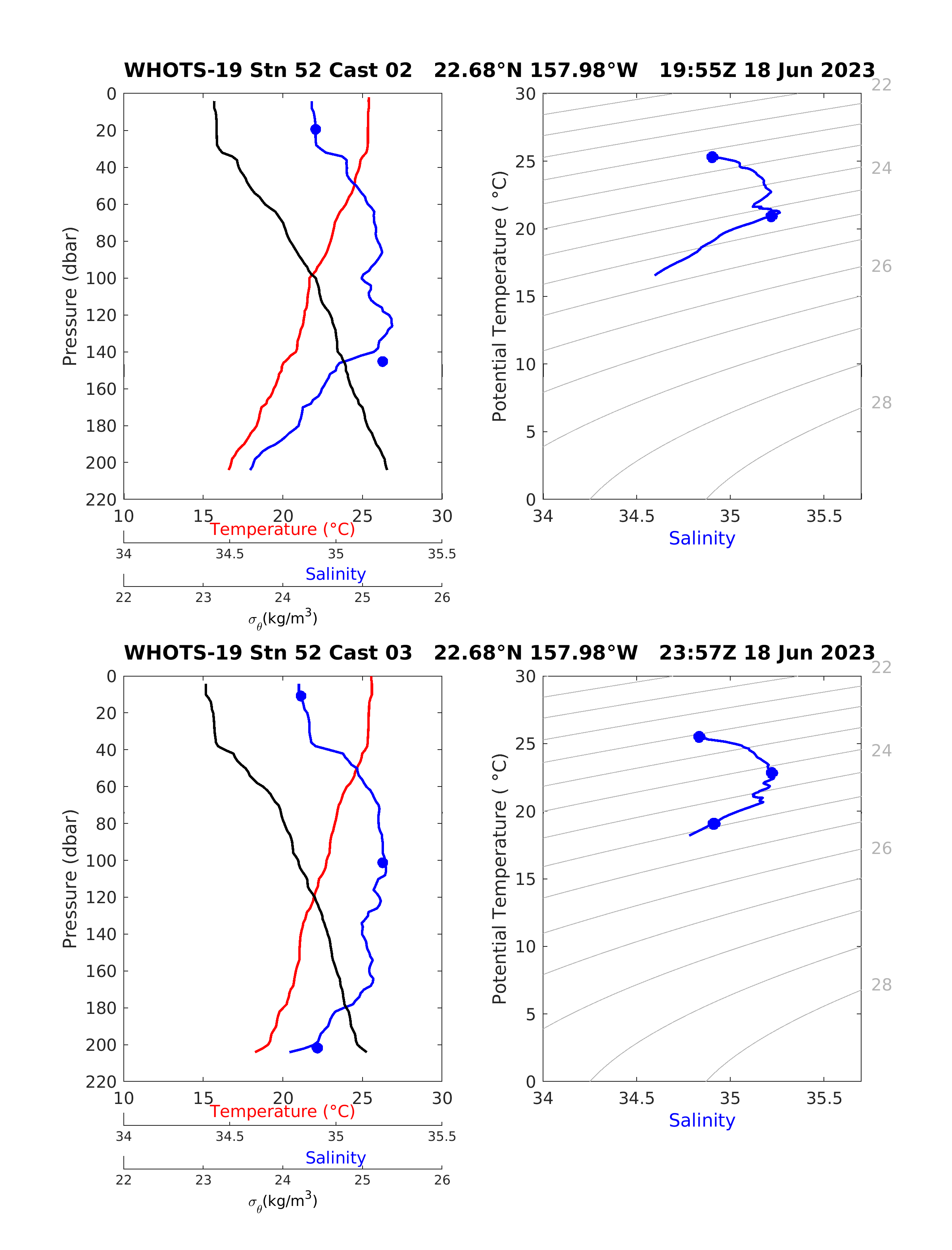
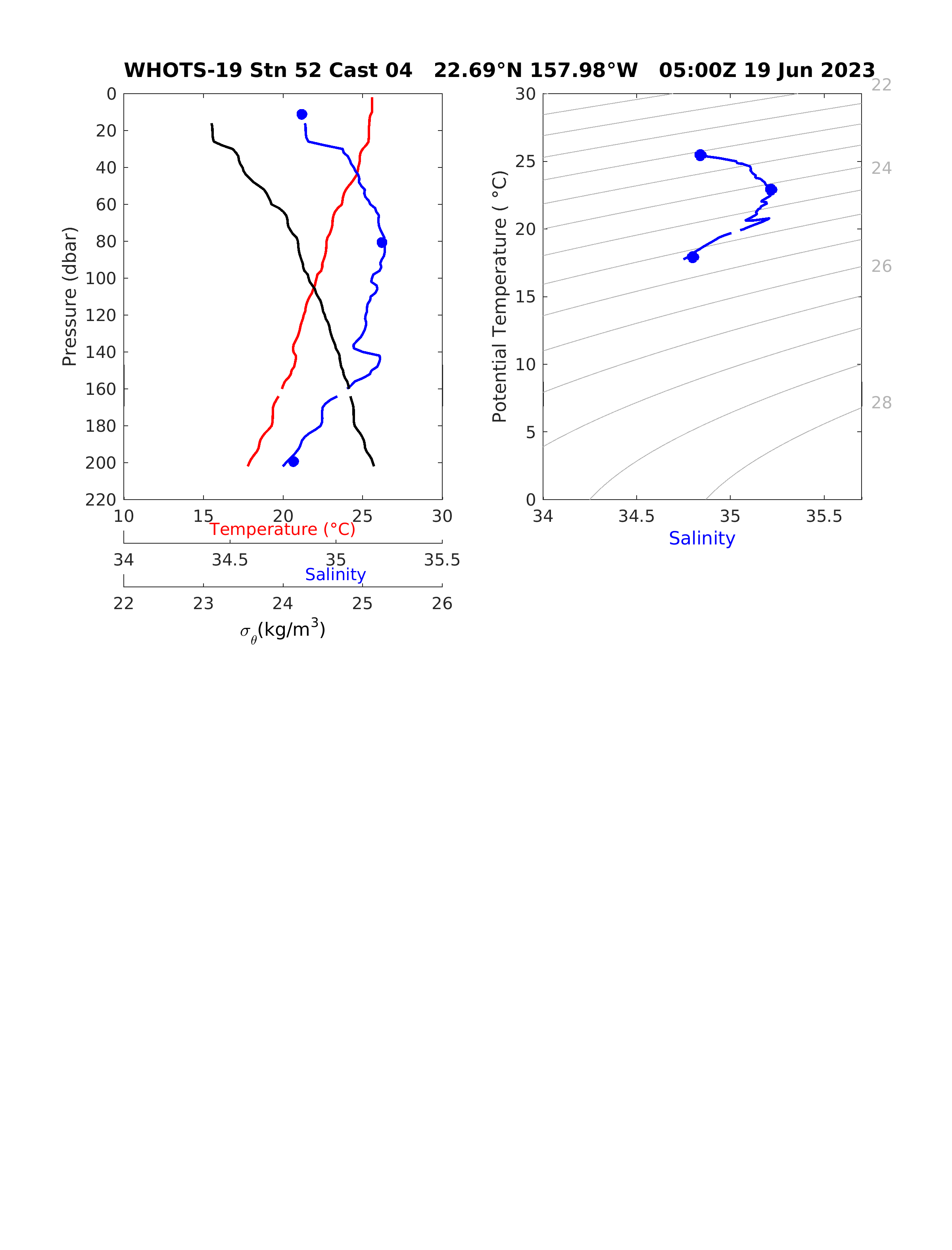
CTD casts conducted near the WHOTS-18 buoy (Station 52) before recovery (Fig. 6.6, Fig. 6.7, Fig. 6.8) displayed a subsurface salinity maximum between 130 and 150 dbar and a mixed layer of about 40 dbar deep.
The temperature MicroCAT records during the WHOTS-18 deployment (Fig. 6.13 through Fig. 6.15) show noticeable seasonal variability in the upper 100 m. A temperature increase in January-February 2023 was evident in all the instruments. The salinity records (Fig. 6.17 through Fig. 6.19) do not show an apparent seasonal cycle, but a sudden drop in salinity was recorded in January 2023, with values mostly below 35 in the upper 40 m for the rest of the deployment. Another salinity drop was recorded by all the instruments after June 2023, reaching 34.5 values in the upper 95 m.
Fig. 6.25 through Fig. 6.27 show contours of the WHOTS-18 MicroCAT data in context with data from the previous 17 deployments. The seasonal cycle is evident in the temperature record, with record temperatures (higher than 26°C) in the summer of 2004, and again in 2014, 2015, 2017, 2019, and 2020. Salinities in the subsurface salinity maximum were relatively low during the first 6 years of the record, only to increase drastically after 2008 through 2015, with some lower salinity episodes in mid-2011 and early 2012. The salinity maximum extended to near the surface in early 2010, 2011, late 2012-early 2013, and February-March 2013. Salinities in the salinity minimum decreased after 2015, showing low salinities above 100 m in 2016, 2017, 2018, and reaching record low values (34.4) in July-August 2019 and July-September 2020. The salinities started to increase after 2021, reaching 35.4 values at the salinity maximum, and extending to the surface in October and November-December 2022. When plotted in \(\sigma\theta\) coordinates (Fig. 6.27), the salinity maximum seems to be centered roughly between 24 and 24.5 \(\sigma\theta\).
Records from the WHOTS-18 MicroCATs (Fig. 6.28) deployed near the bottom of the mooring (4710 m) detected temperature and salinity changes related to episodic ‘cold events’ apparently caused by bottom water moving between abyssal basins [Lukas et al., 2001]. These events are being monitored by instruments at the ALOHA Cabled Observatory (ACO) [Howe et al., 2011] , a deep water observatory located at the bottom of Station ALOHA (about 6 nautical miles north from the WHOTS-18 anchor), since June 2011. Fig. 6.28 shows temperature and salinity records from the WHOTS-18 MicroCATs superimposed on the ACO data. The MicroCAT data agreed with the temperature decrease and the salinity variability registered by ACO instruments during a cold event in August 2022, and during minor events in October 2022 and late February 2023.
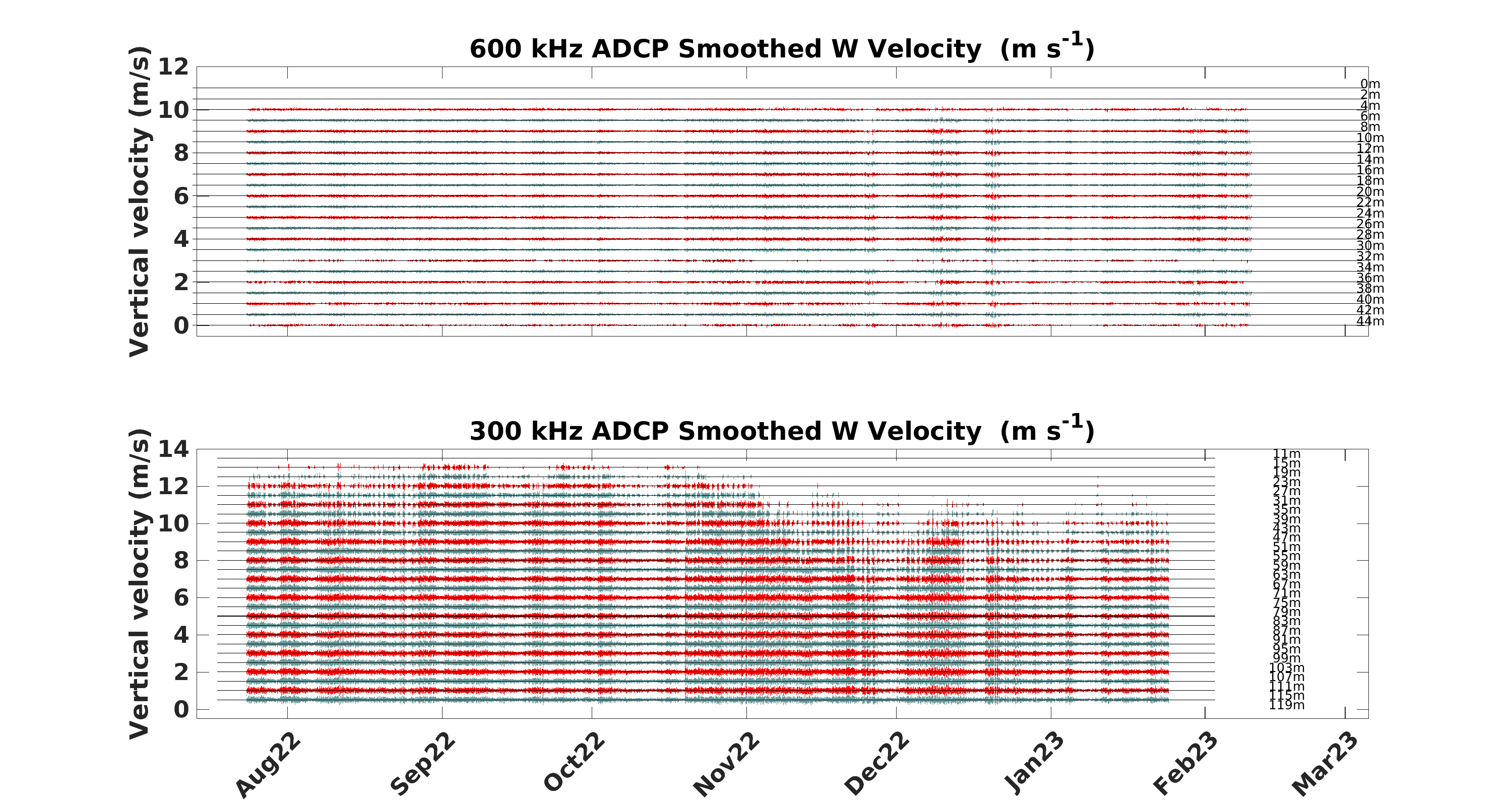
Fig. 6.31 through Fig. 6.33 shows the time series of the zonal, meridional, and vertical currents recorded with the moored ADCPs during the WHOTS-18 deployment. Fig. 6.29 shows the ADCP current components’ contours in context with data from the previous deployments. Despite the gaps in the data, an apparent variability is seen in the zonal and meridional currents, apparently caused by passing eddies. There have been periods of intermittent positive or negative zonal currents on top of this variability, for instance, during 2007-2008. The contours of the vertical current component show a transition in the magnitude of the contours near 47 m, indicating that the 300 kHz ADCP located at 126 m moves more vertically than the 600 kHz ADCP located at 47.5 m.
A comparison between the moored ADCP data and the shipboard ADCP data obtained during the WHOTS-18 cruise is shown in Fig. 6.34, and Fig. 6.35. A similar comparison during the WHOTS-19 cruise was not possible because both moored ADCPs stopped working before the mooring was recovered. The shipboard ADCP data during the WHOTS-19 cruise are shown in Fig. 6.36 and Fig. 6.37. Some differences were seen during the WHOTS-18 cruise comparisons, especially in the zonal component, maybe due to the mooring motion, which was not removed from the data. Comparisons between the available shipboard ADCP from HOT-339 to -342 cruises and the mooring data are shown in Fig. 6.38 through Fig. 6.39.
The Xeos-GPS receiver registered the WHOTS-18 buoy motion, and its positions are plotted in Fig. 6.41. The buoy remained predominantly around its intended deployment location, with noticeable variability both in latitude and longitude, particularly during the periods from November 2022 to March 2023. The power spectrum of these data Fig. 6.43) shows significant energy at the diurnal (K1) and semidiurnal (M2) tidal frequencies, indicating that tidal forces were a major driver of the buoy’s movement. Combining the buoy motion with the tilt (a combination of pitch and roll) from the ADCP data (Fig. 6.43) showed that the tilt increased as the buoy’s distance from the anchor increased. This was expected since the inclination of the cable increases as the buoy moves farther from the anchor.
6.1. CTD Profiling Data
Profiles of temperature, salinity, and potential density (\(\sigma\theta\)) from the casts obtained during the WHOTS-18 deployment cruise are presented in Fig. 6.1 through Fig. 6.5, together with the results of bottle determination of salinity. Fig. 6.6 through Fig. 6.8 shows the results of the CTD profiles during the WHOTS-19 cruise.
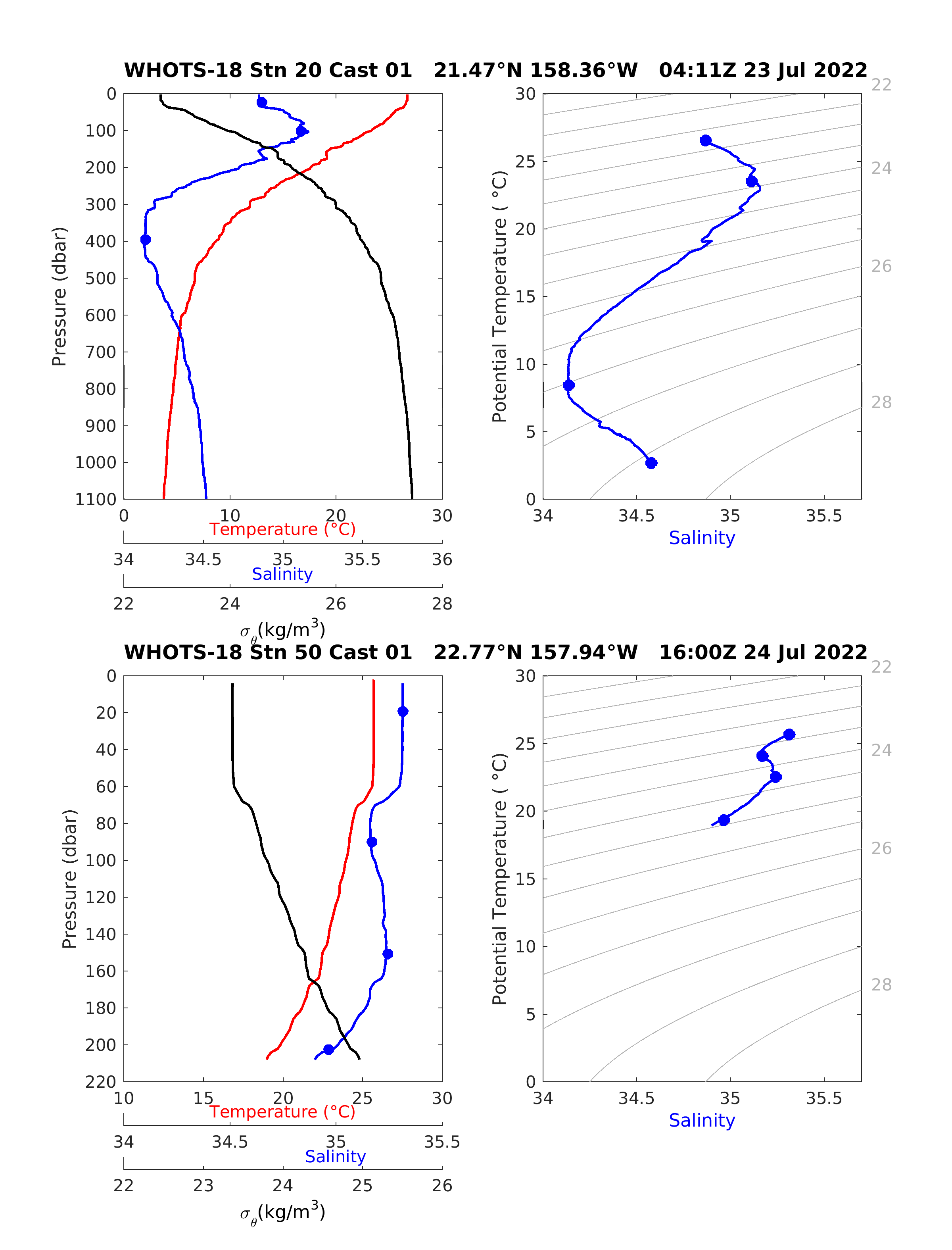
Fig. 6.1 [Upper left panel] Profiles of CTD temperature, salinity, and potential density (\(\sigma\theta\)) as a function of pressure, including discrete bottle salinity samples (when available) for station 20 cast 1 during the WHOTS-18 cruise. [Upper right panel] Profiles of CTD salinity as a function of potential temperature, including discrete bottle salinity samples (when available) for station 20 cast 1 during the WHOTS-18 cruise. [Lower left panel] Same as in the upper left panel, but for station 50 cast 1. [Lower right panel] Same as in the upper right panel, but station 50 cast 1.
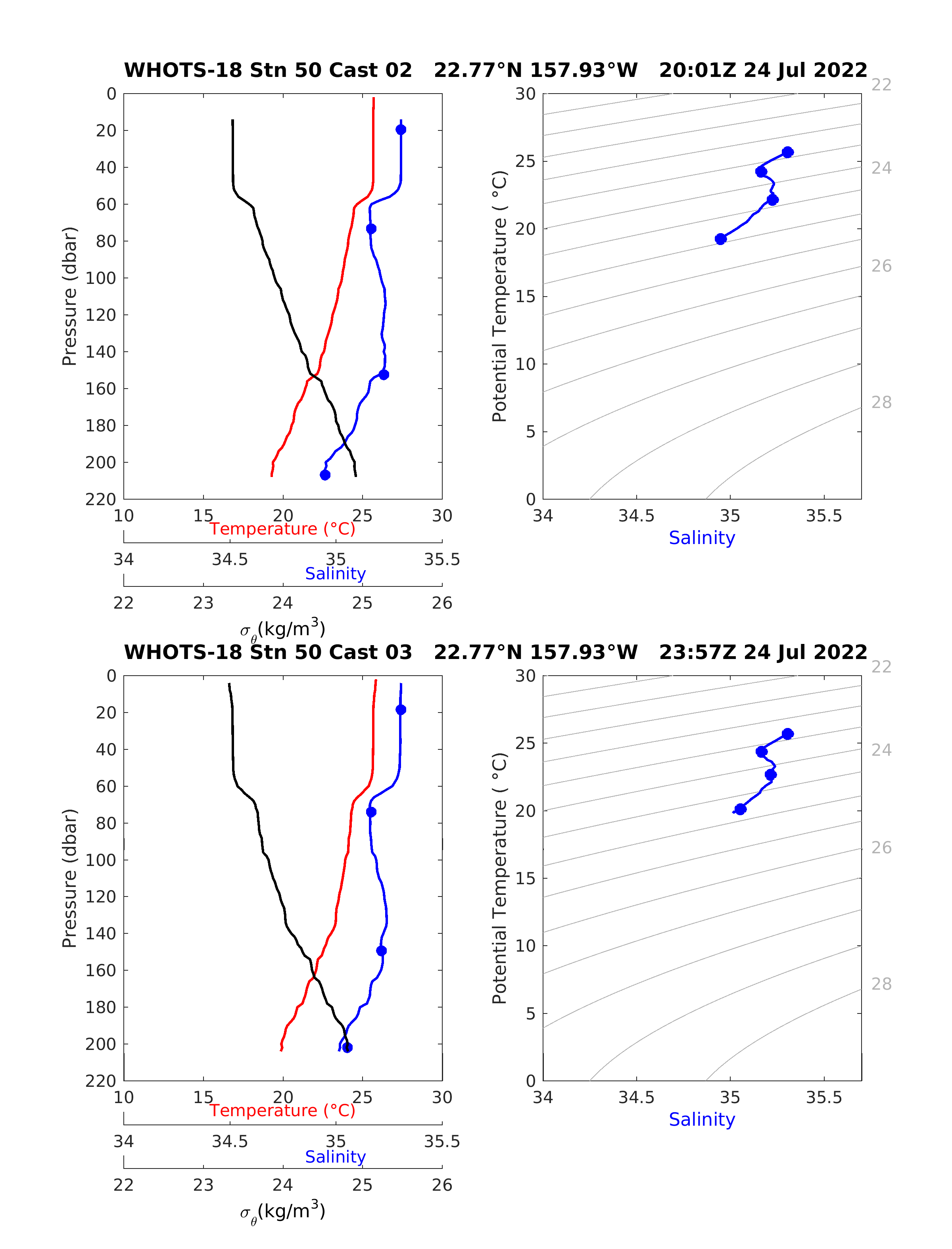
Fig. 6.2 [Upper panels] Same as in Fig. 6.1, but for station 50, cast 2. [Lower panels] Same as Fig. 6.1, but for station 50, cast 3.
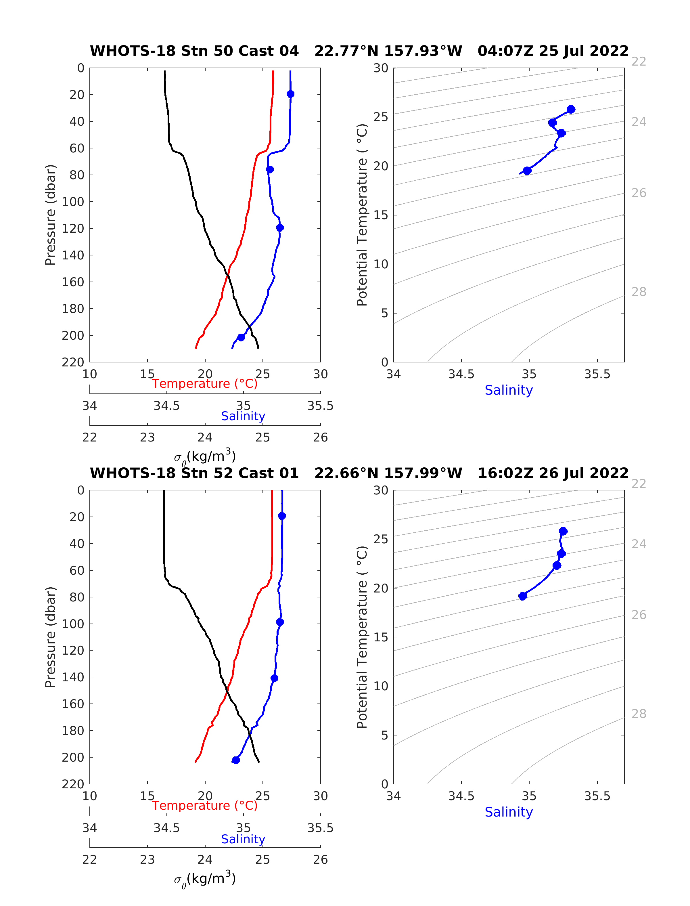
Fig. 6.3 [Upper panels] Same as in Fig. 6.1, but for station 50, cast 4. [Lower panels] Same as in Fig. 6.1, but for station 52 cast 1.
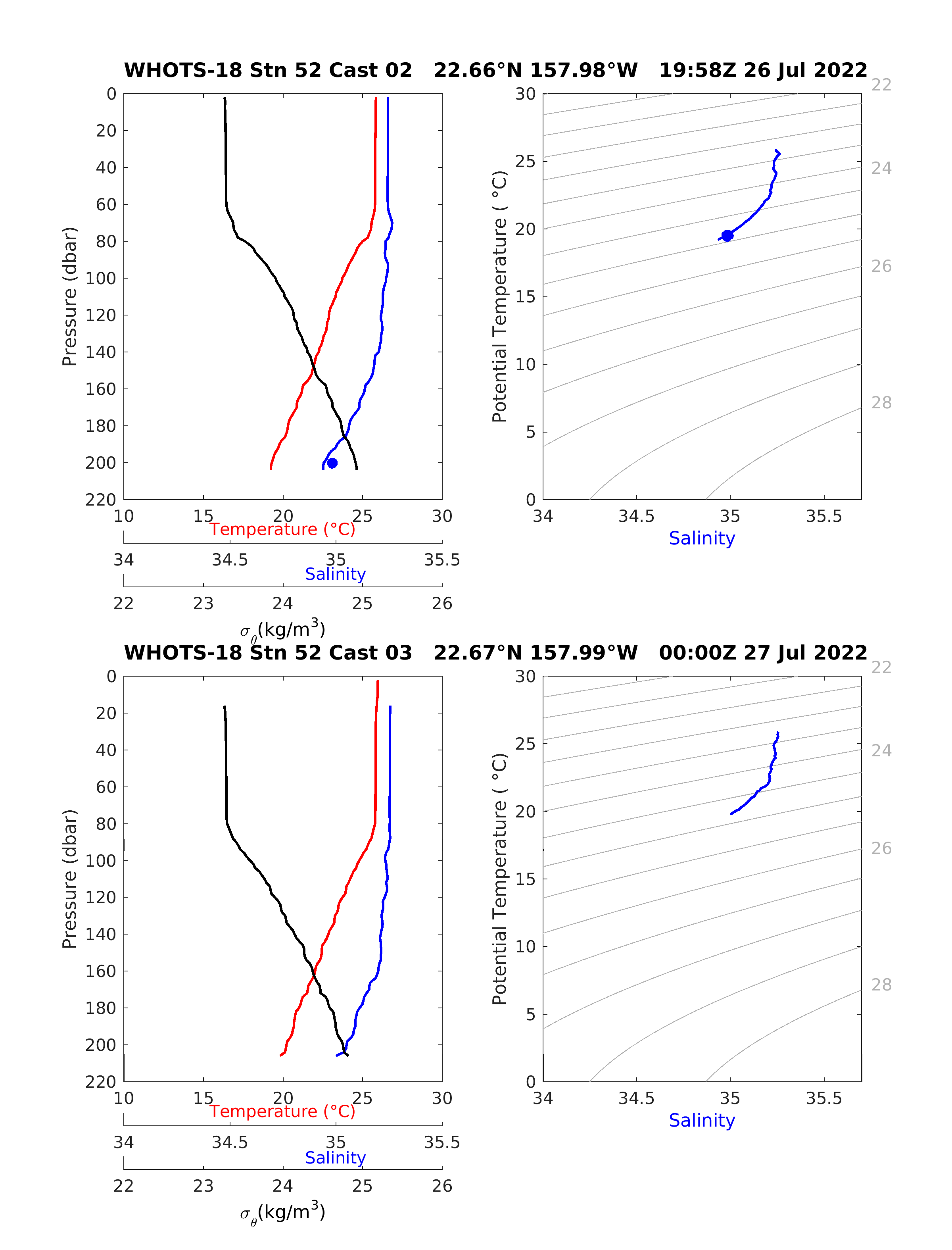
Fig. 6.4 [Upper panels] Same as in Fig. 6.1, but for station 52, cast 2. [Lower panels] Same as in Fig. 6.1, but for station 52, cast 3.
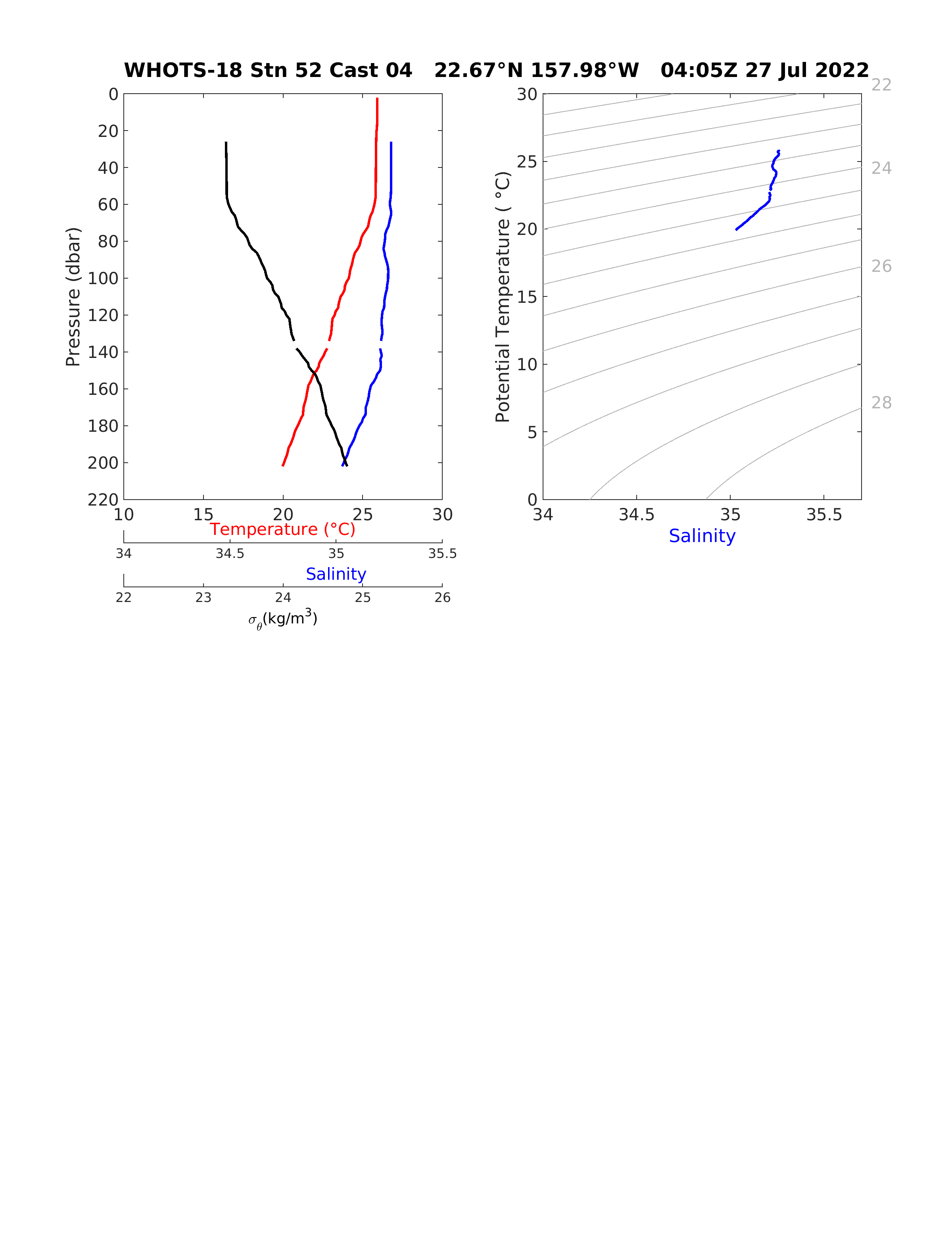
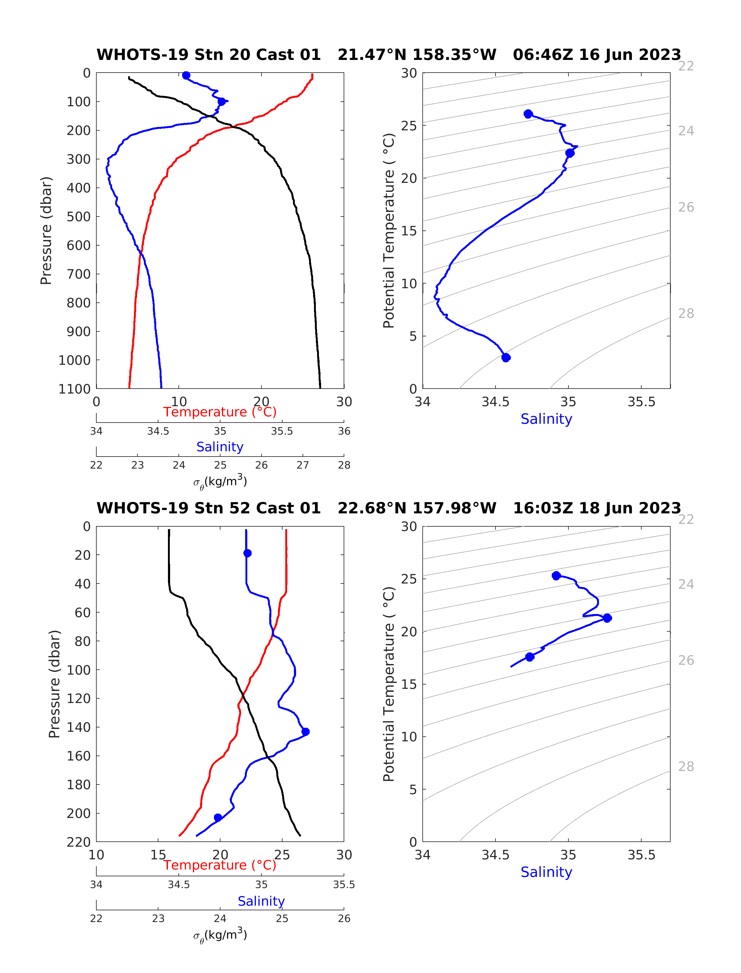
Fig. 6.6 [Upper left panel] Profiles of CTD temperature, salinity, and potential density (\(\sigma\theta\)) as a function of pressure, including discrete bottle salinity samples (when available) for station 20 cast 1 during the WHOTS-19 cruise. [Upper right panel] Profiles of CTD salinity as a function of potential temperature, including discrete bottle salinity samples (when available) for station 20 cast 1 during the WHOTS-19 cruise. [Lower left panel] Same as in the upper left panel, but for station 52 cast 1. [Lower right panel] Same as in the upper right panel, but station 52 cast 1.
6.2. Thermosalinograph Data
Underway measurements of near-surface temperature and salinity from the thermosalinograph (TSG) system on board the R/V Oscar Sette cruise are presented in Fig. 6.9 and navigational data is shown in Fig. 6.10 for the WHOTS-18 cruise. TSG and navigational data during the WHOTS-19 cruise, on board the R/V Oscar Sette, are presented in Fig. 6.11 and Fig. 6.12, respectively.
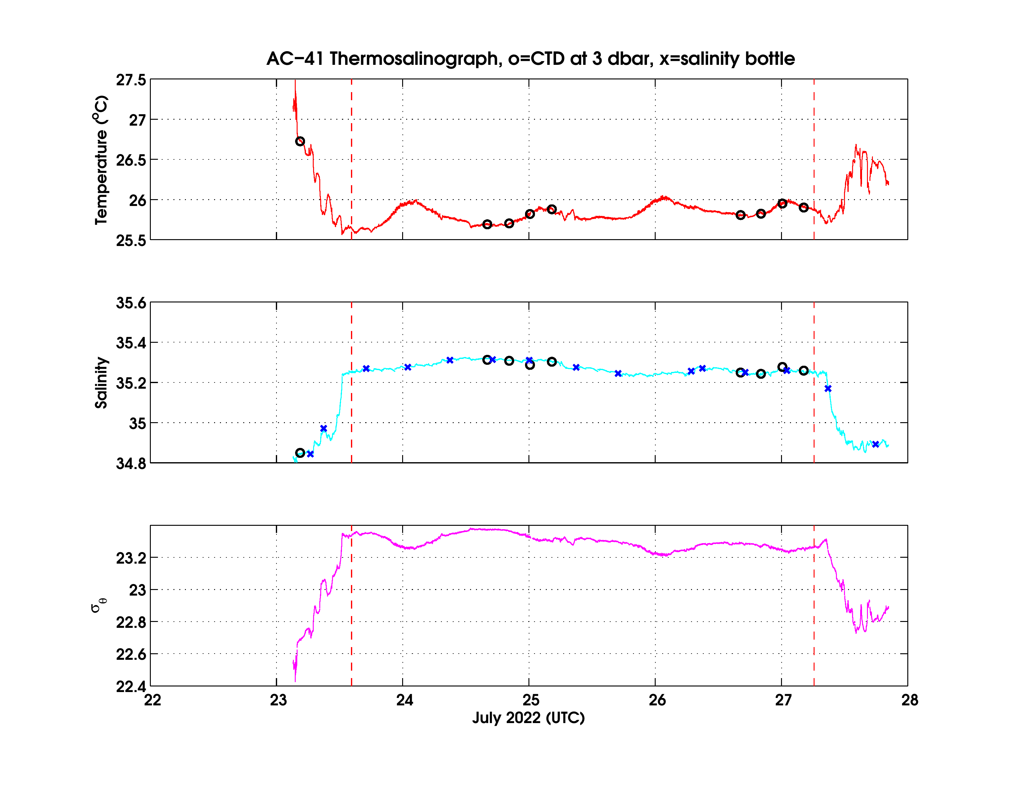
Fig. 6.9 Final processed temperature (upper panel), salinity (middle panel), and potential density (\(\sigma\theta\)) (lower panel) data from the continuous underway system onboard the R/V Hi’ialakai during the WHOTS-18 cruise. Temperature and salinity taken from 6-dbar CTD data (circles) and salinity bottle sample data (crosses) are superimposed. The dashed vertical red line indicates the period of occupation of Station ALOHA and the WHOTS site.
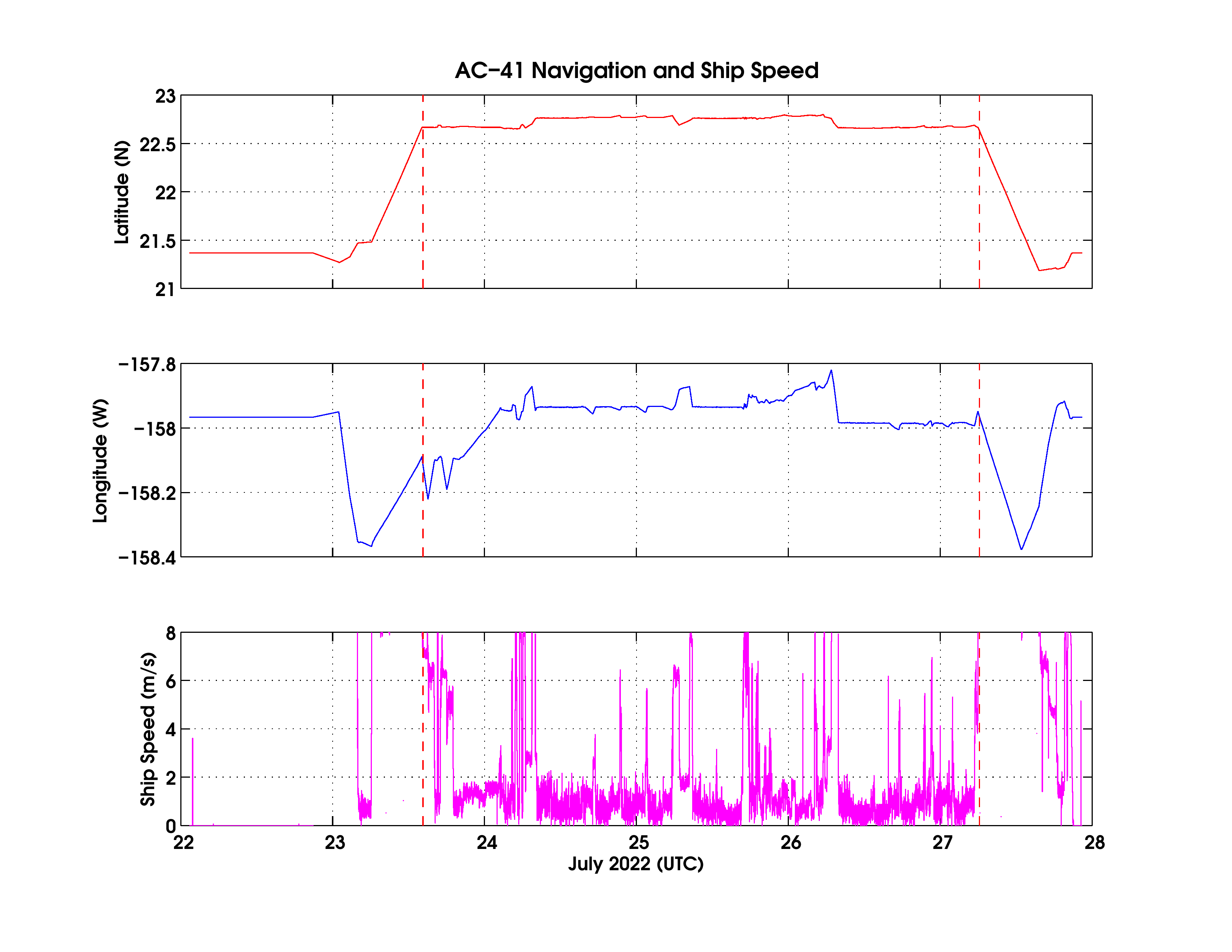
Fig. 6.10 Timeseries of latitude (upper panel), longitude (middle panel), and ship’s speed (lower panel) during the WHOTS-18 cruise.
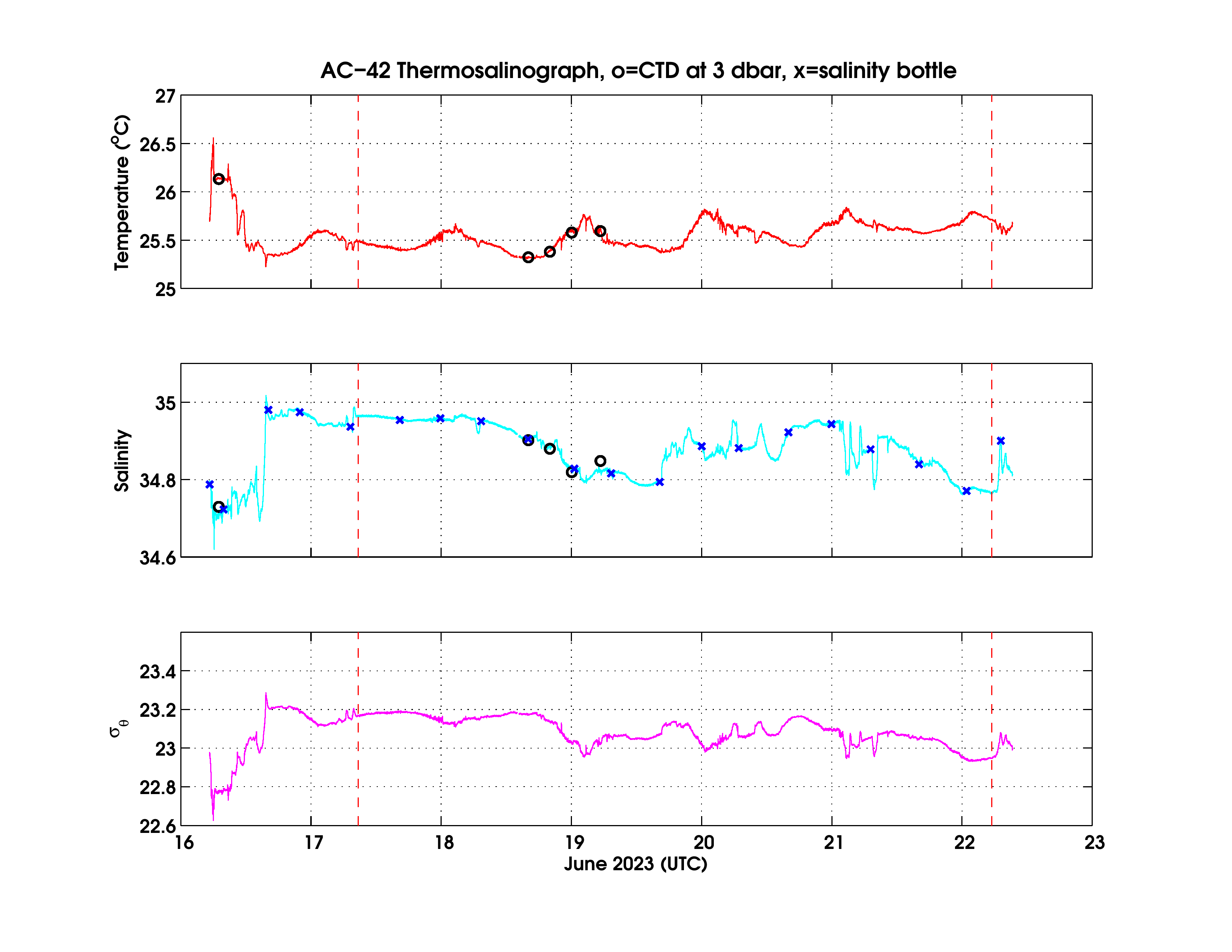
Fig. 6.11 Final processed temperature (upper panel), salinity (middle panel), and potential density (\(\sigma\theta\)) (lower panel) data from the continuous underway system onboard the R/V Oscar Sette during the WHOTS-19 cruise. Temperature and salinity were taken from 6-dbar CTD data (circles), and salinity bottle sample data (crosses) are superimposed. The dashed vertical red line indicates the period of occupation of Station ALOHA and the WHOTS site.
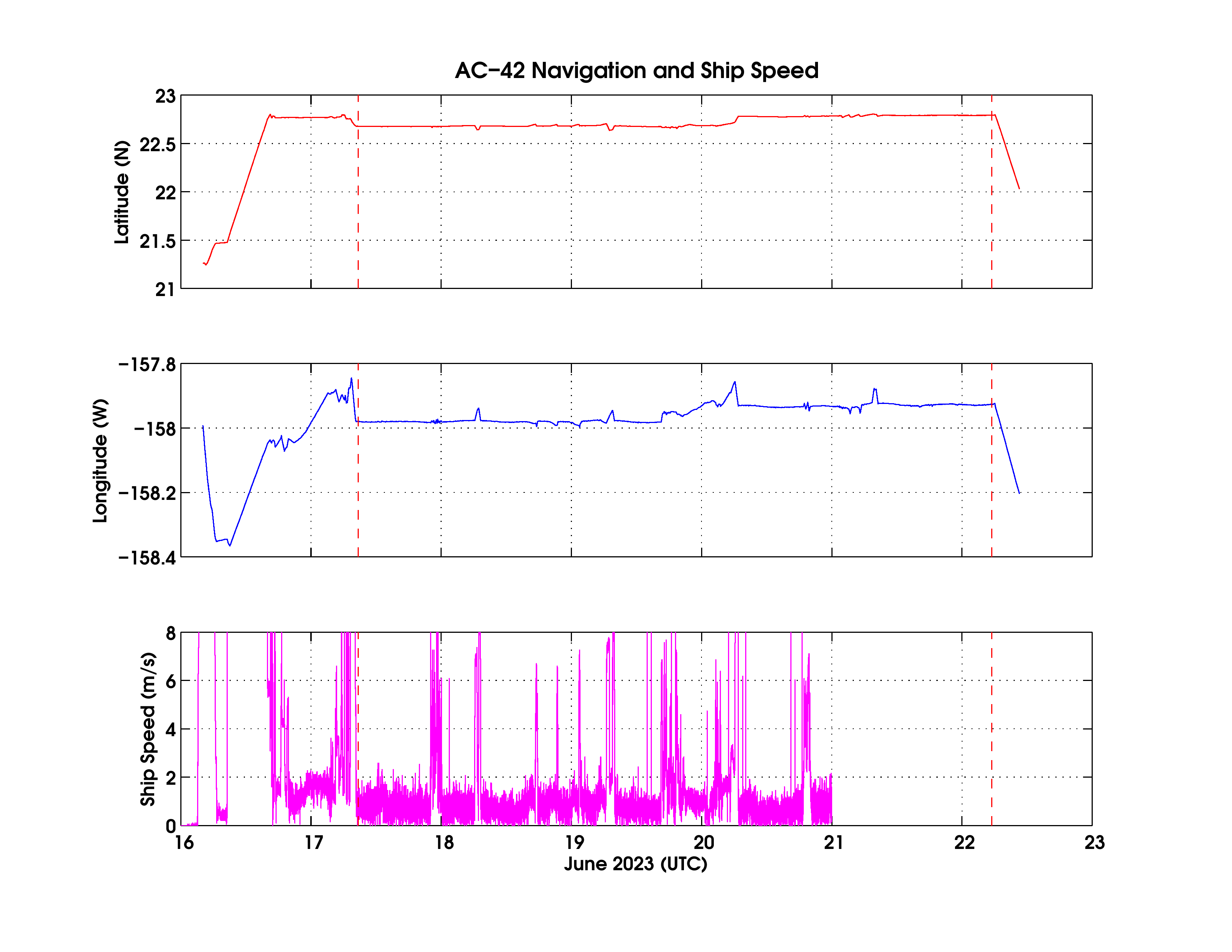
Fig. 6.12 Timeseries of latitude (upper panel), longitude (middle panel), and ship’s speed (lower panel) during the WHOTS-19 cruise.
6.3. MicroCAT Data
The temperatures measured by MicroCATs during the mooring deployment for WHOTS-18 are presented in Fig. 6.13 through Fig. 6.16 for each of the depths where the instruments were located. The salinities are plotted in Fig. 6.17 through Fig. 6.20. The potential densities (\(\sigma\theta\)) are plotted in Fig. 6.21 through Fig. 6.24.
Contoured plots of temperature and salinity as a function of depth for the deployments WHOTS-1 through -18 are presented in Fig. 6.25, and contoured plots of potential density (\(\sigma\theta\)) as a function of depth are in Fig. 6.26, and of salinity as a function of \(\sigma\theta\) are in Fig. 6.27.
The potential temperature (\(\theta\)) and salinity measured by the deep MicroCATs during the mooring deployment are shown in Fig. 6.28. Also shown in the plot are the \(\theta\) and salinity data obtained with a MicroCAT (SBE-37) installed in the ALOHA Cabled Observatory, about six nautical miles north from the WHOTS-18 anchor. The instrument is located 2 m above the bottom.
Fig. 6.13 Temperatures from MicroCATs during WHOTS-18 deployment at 1.5, 7, 15, and 25m.
Fig. 6.17 Salinities from MicroCATs during WHOTS-18 deployment at 1.5, 7, 15, and 25m
Fig. 6.21 Potential densities (\(\sigma\theta\)) from MicroCATs during WHOTS-18 deployment at 1.5, 7, 15, and 25m.

Fig. 6.25 Contour plots of temperature (upper panel) and salinity (lower panel) versus depth from SeaCATs/MicroCATs during WHOTS-1 through WHOTS-18 deployments. The shaded areas indicate missing data. The diamonds along the right axis indicate the depths of the instrument.

Fig. 6.26 Contour plots of potential density (\(\sigma\theta\)), versus depth from SeaCATs/MicroCATs during WHOTS-1 through WHOTS-18 deployments. The shaded areas indicate missing data. The diamonds along the right axis in the upper figure indicate the depths of the instrument.
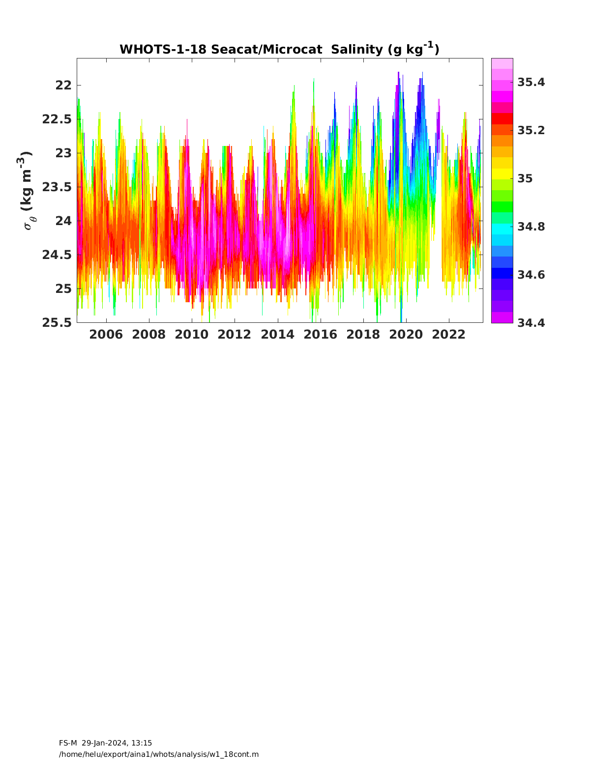
Fig. 6.27 Contour plots of salinity versus \(\sigma\theta\) from SeaCATs/MicroCATs during WHOTS-1 through WHOTS-18 deployments.
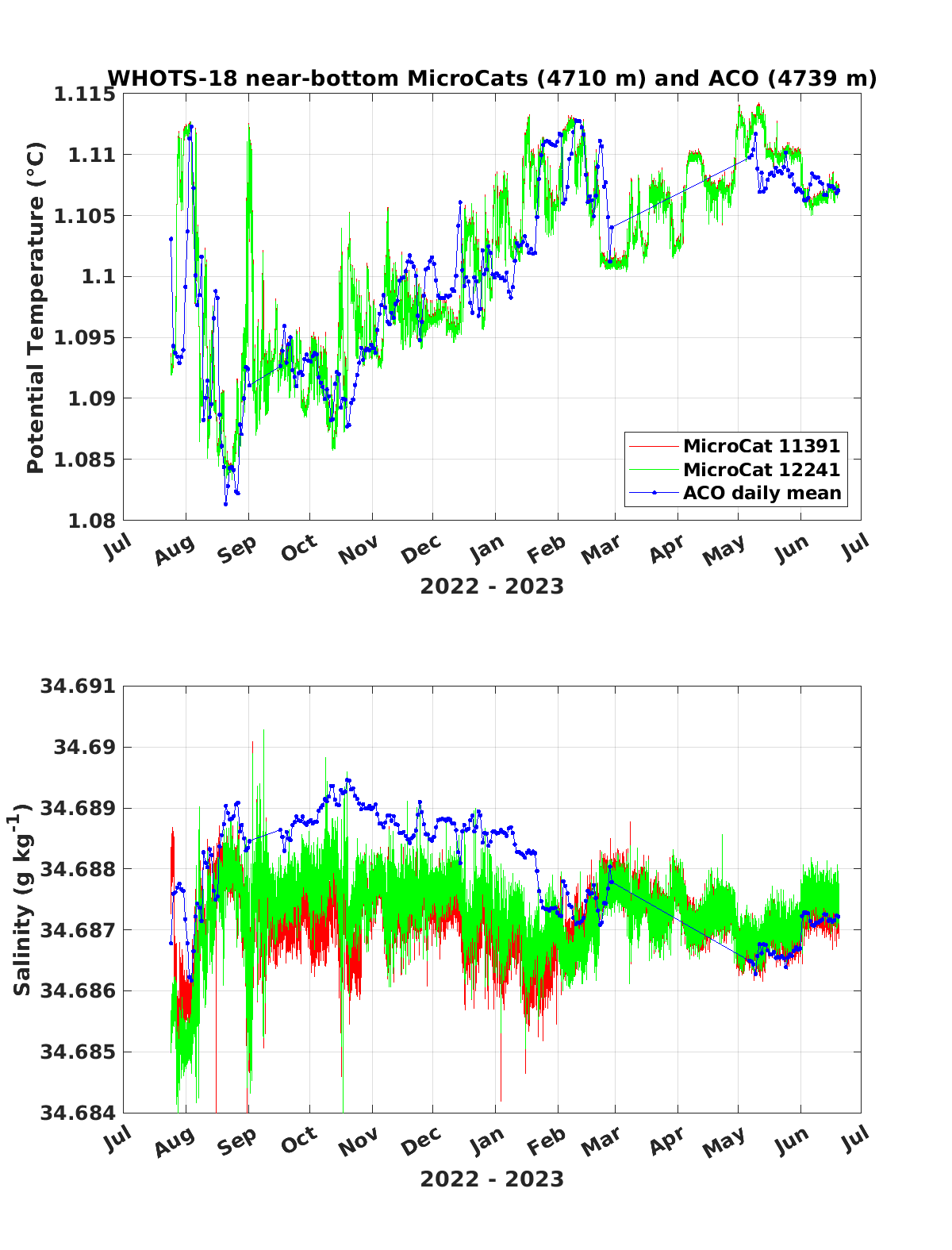
Fig. 6.28 Potential temperature (upper panel) and salinity (lower panel) time-series from the ALOHA Cabled Observatory (ACO) sensors and the WHOTS-18 MicroCATs 11391 and 12241.
6.4. Moored ADCP Data
The contour plots presented in Fig. 6.29 illustrate the temporal evolution of the smoothed horizontal (zonal and meridional components) and vertical velocity as a function of depth for the WHOTS mooring deployments from WHOTS 1 through WHOTS 18. The zonal velocity shows seasonal variability, with alternating eastward and westward flows often observed down to 100 meters. Notable changes are evident particularly during the deployments from 2010 to 2012 and from 2018 to 2020, where shifts in both magnitude and direction are prominent. The meridional component displays considerable variability in northward and southward flow, with the most significant changes occurring between 2011 and 2013. The vertical velocity component remains weaker overall, but increased variability is noticeable during the 2011 to 2013 period and again from 2018 onward.
These observations highlight key periods of variability and provide insights into the evolving current structure throughout the WHOTS deployments. The years 2011-2013 and 2018-2020 stand out as periods with significant changes in both horizontal and vertical velocity patterns.
The vertical velocity component is relatively weak compared to the horizontal components, indicating minimal large-scale vertical movement. However, slight positive and negative velocities during specific periods suggest internal wave activity or localized vertical mixing events.
The plots in Fig. 6.30 detail the WHOTS-18 ADCP velocity measurements from mid-2022 through early 2023. The zonal velocity exhibits a predominantly westward flow throughout the deployment, with occasional eastward anomalies observed in the late summer and early winter months. These patterns align with seasonal wind forcing and possibly localized wind-driven upwelling events. The meridional velocity reveals alternating periods of northward and southward movement, suggesting the influence of mesoscale eddies and regional circulation patterns that drive variability along the meridional axis. In particular, significant northward transport was observed during late 2022, which transitioned to a southward direction in early 2023.
The vertical velocity component is relatively weak compared to the horizontal components, indicating minimal large-scale vertical movement, consistent with the stratified nature of the upper ocean at these depths. However, slight positive and negative velocities during specific periods suggest internal wave activity or localized vertical mixing events.
These plots collectively help us understand the dynamics of the ocean at the WHOTS-18 site, highlighting the importance of the combined influence of local wind forcing, mesoscale eddy activity, and internal waves in shaping the observed current structure.
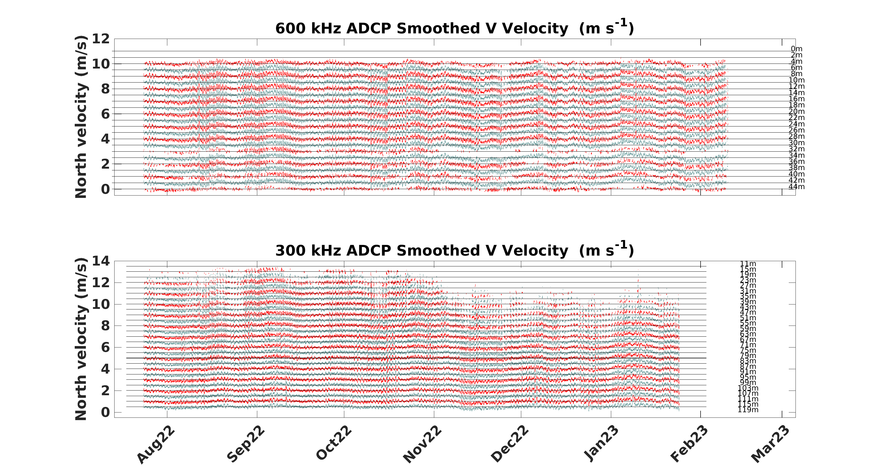
A staggered time-series of smoothed horizontal and vertical velocities are shown in Fig. 6.31 through Fig. 6.33. Smoothing was performed by applying a daily running mean to the data and then interpolating it on an hourly grid.
Contours of east and north velocity components from the Ship Oscar Sette Ocean Surveyor broadband 75 kHz shipboard ADCP, and the moored 300 kHz ADCP from the WHOTS-18 deployment as a function of time and depth, during the WHOTS-18 cruise, are shown in Fig. 6.34 and Fig. 6.35.

Fig. 6.29 Contour plot of east velocity component (\(m s^{-1}\)) versus depth and time from the moored ADCPs from the WHOTS-1 through -18 deployments (upper panel). Contour plot of north velocity component (\(m s^{-1}\)) (middle panel). Contour plot of vertical velocity component (\(m s^{-1}\))(lower panel).
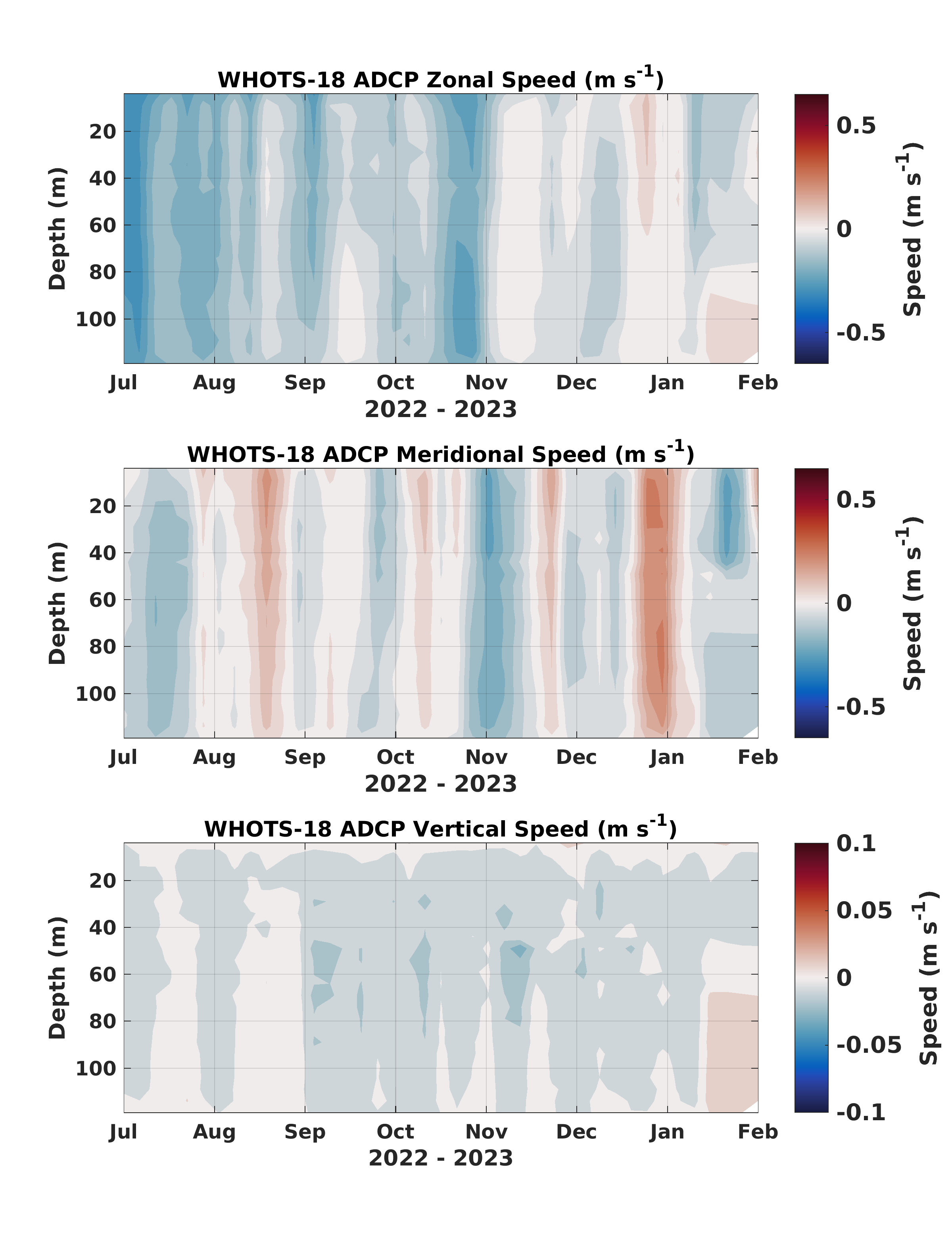
Fig. 6.30 Contour plot of east velocity component (\(m s^{-1}\)) versus depth and time from the moored ADCP WHOTS-18 (upper panel). Contour plot of north velocity component (\(m s^{-1}\)) (middle panel). Contour plot of vertical velocity component (\(m s^{-1}\))(lower panel).
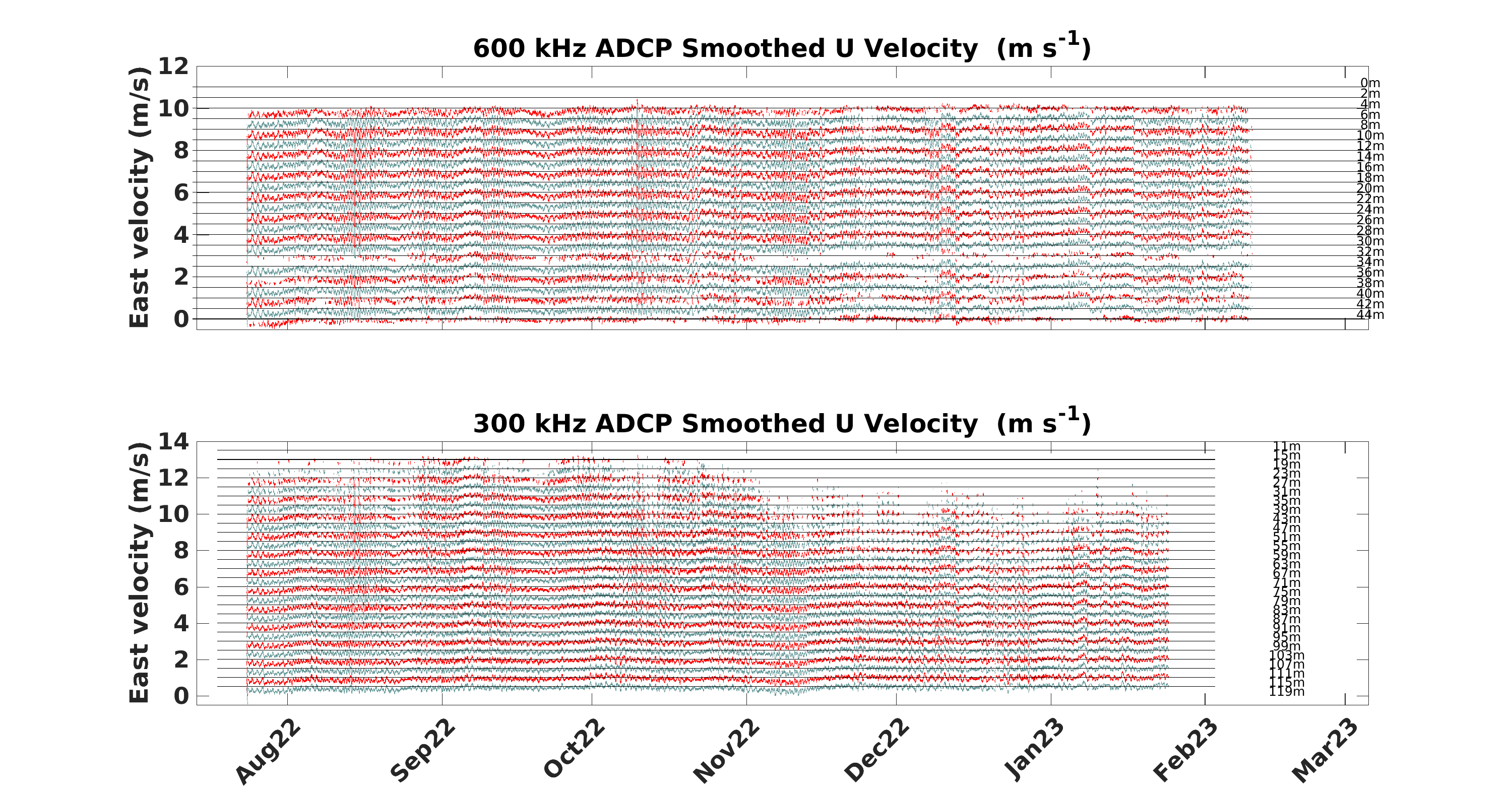
Fig. 6.31 Staggered time-series of east velocity component (\(m s^{-1}\)) for each bin of the 600 kHz (upper panel) and 300 kHz (lower panel) moored ADCPs during WHOTS-18. The time-series are offset upwards by 0.5 \(m s^{-1}\); each bin’s depth is on the right.
6.5. Moored and Shipboard ADCP comparisons
The contour plots in Fig. 6.34, and Fig. 6.35 present a comparison of the zonal and meridional current components captured by both the shipboard 75 kHz ADCP from the Oscar Sette and the moored 300 kHz ADCP at the WHOTS-18 mooring site. These plots provide insights into the consistency and discrepancies between shipboard and moored ADCP measurements throughout the WHOTS-18 cruise. Similar moored ADCP comparisons with the WHOTS-19 cruise shipboard ADCP (Fig. 6.36, and Fig. 6.37) were not possible because the moored ADCPs stopped working before the mooring was recovered.
6.5.1. WHOTS-18 Deployment Comparison
For the WHOTS-18 cruise (as shown in Fig. 6.34 and Fig. 6.35), the shipboard ADCP data from the Oscar Sette and the moored ADCP data reveal certain distinctions between zonal and meridional velocities at similar depths. Notably, the zonal current data show consistent eastward and westward oscillations between both ADCPs, though the magnitude appears more pronounced in the shipboard ADCP, particularly around late July 2022. These differences may be influenced by the positioning of the moored ADCP relative to the ship’s track and its response to localized eddies or current variations.
The meridional current comparison (as presented in Fig. 6.35) also displays variations between the two datasets. The moored ADCP, being positioned at a fixed depth, captures consistent northward and southward patterns, whereas the shipboard ADCP data exhibit more fluctuation at shallower depths, potentially linked to local surface current variability during the cruise. The variability is especially pronounced around late July 2022, which aligns with the timing of increased dynamic activity also observed in the zonal component.
6.5.2. WHOTS-19 Deployment Comparison
WHOTS-19 cruise shipboard ADCP zonal and meridional currents are shown in Fig. 6.36 and Fig. 6.37. The zonal current reveals a predominantly westward flow throughout the deployment period, with occasional eastward pulses, particularly around day 168 and day 169. The eastward flow on day 168 is concentrated mainly between 40 to 100 m. Other eastward flows appear prominently at different times during the deployment.
The meridional current displays alternating northward and southward flows, which are more variable compared to the zonal currents. Between day 168 and day 169, there is a transition from predominantly southward flow to mixed northward and southward patterns, particularly in the upper 70 meters. Below 70 meters, the variability in meridional flow becomes less pronounced, with smoother transitions between northward and southward flows.
As mentioned above, the 300 kHz and the 600 kHz moored ADCP experienced operational failures, and we couldn’t make a direct comparison between the Shipboard ADCP and Moored ADCP data for the WHOTS-19 deployment cruise. The 300 kHz instrument stopped recording on January 24, 2023, and the 600 kHz instrument stopped on February 10, 2023, likely due to power loss caused by bulkhead corrosion. As a result, only the shipboard ADCP data is available for the WHOTS-19 cruise analysis, limiting the ability to cross-verify these measurements with the moored instruments.
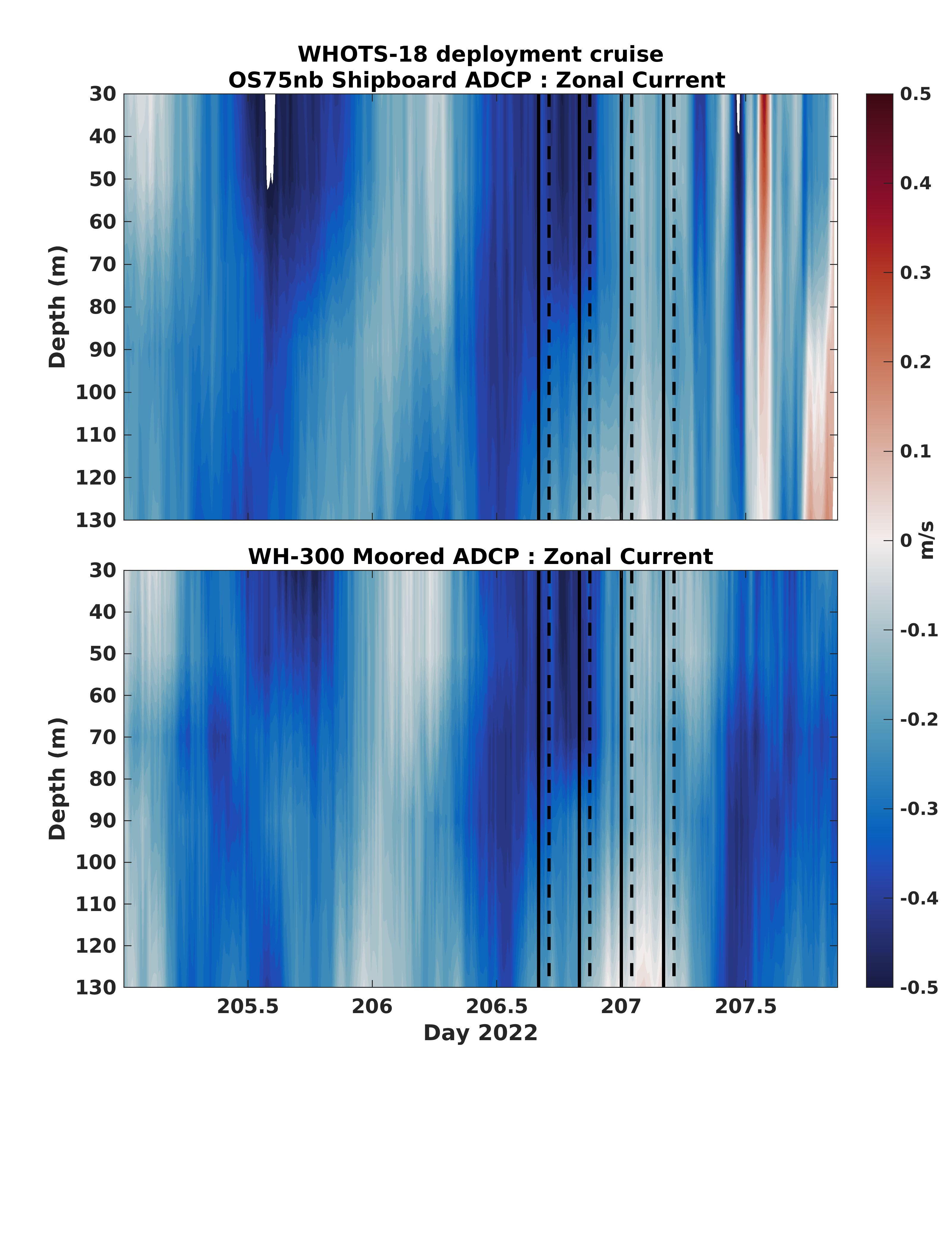
Fig. 6.34 The contour of zonal currents (\(m s^{-1}\)) from the Ship Oscar Sette Ocean Surveyor narrowband 75 kHz shipboard ADCP (upper panel), and the moored 300 kHz ADCP from the WHOTS-18 mooring (bottom panel) as a function of time and depth, during the WHOTS-18 cruise. Times when the CTD rosette was in the water are identified between solid and dashed black lines.
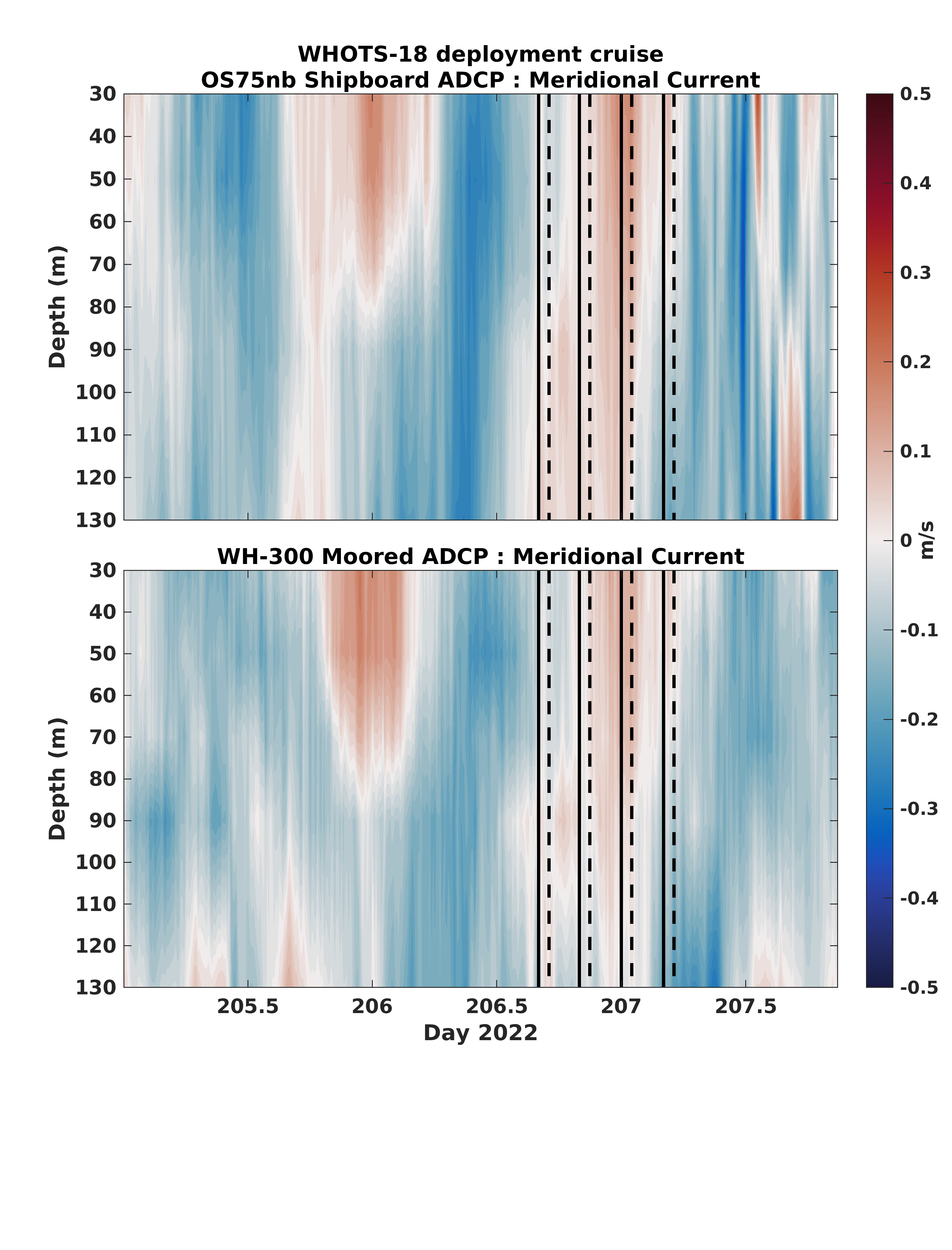
Fig. 6.35 The contour of meridional currents (\(m s^{-1}\)) from the Ship Oscar Sette Ocean Surveyor narrowband 75 kHz shipboard ADCP (upper panel), and the moored 300 kHz ADCP from the WHOTS-18 mooring (bottom panel) as a function of time and depth, during the WHOTS-18 cruise. Times when the CTD rosette was in the water are identified between solid and dashed black lines.
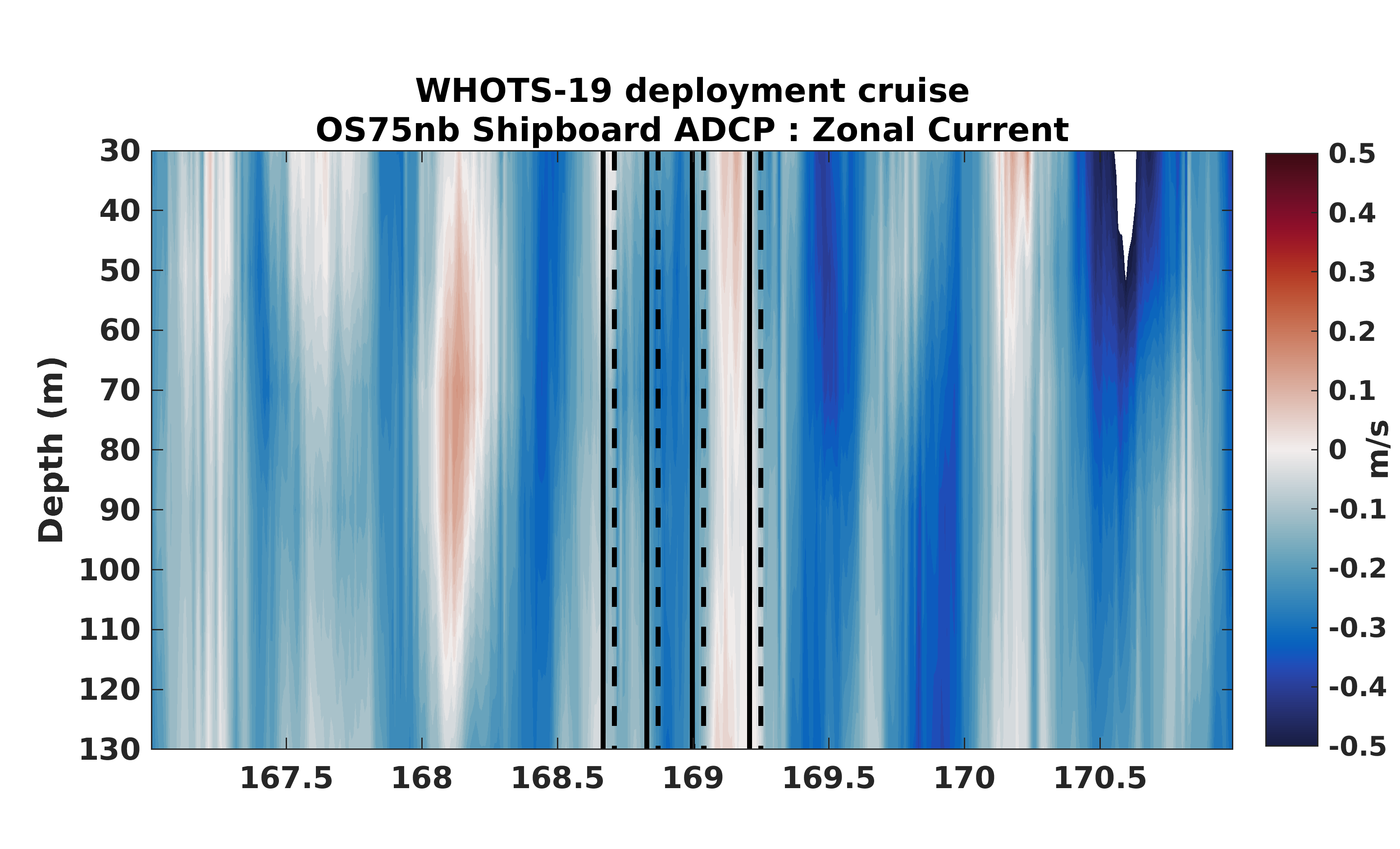
Fig. 6.36 The contour of zonal currents (\(m s^{-1}\)) from the Ship Oscar Sette Ocean Surveyor narrowband 75 kHz shipboard ADCP as a function of time and depth, during the WHOTS-19 cruise. Times when the CTD rosette was in the water are identified between solid and dashed black lines.
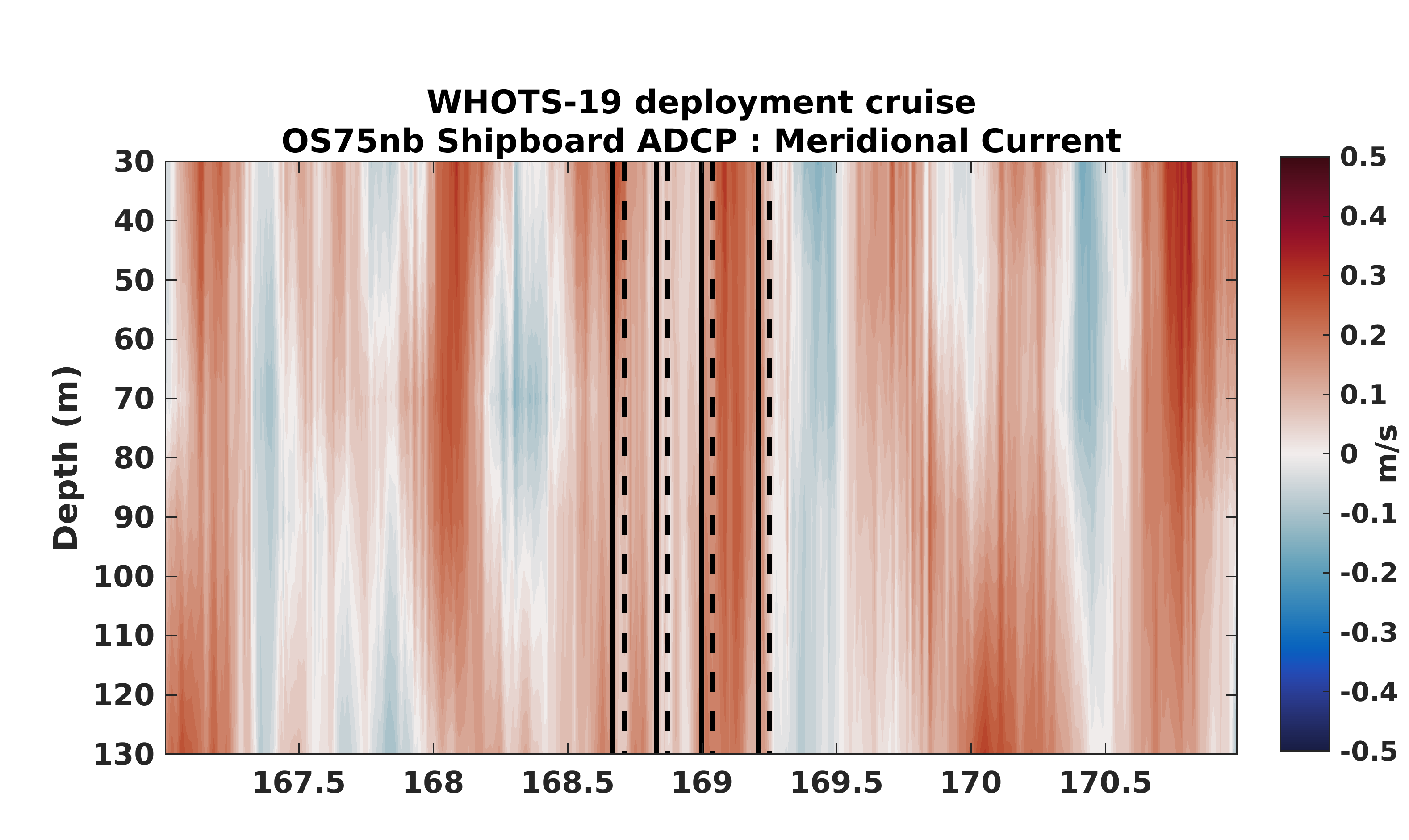
Fig. 6.37 Contours of meridional currents (\(m s^{-1}\)) from the Ship Oscar Sette Ocean Surveyor narrowband 75 kHz shipboard ADCP as a function of time and depth, during the WHOTS-19 cruise. Times when the CTD/rosette was in the water are identified between the solid and dashed black lines.
Comparisons between quality-controlled moored ADCPs during the WHOTS-18 deployment and available shipboard ADCP obtained during regular HOT cruises 338 to 342, and during the mooring deployment (WHOTS-18) and recovery (WHOTS-19) cruises are shown in Fig. 6.38 for the 300 kHz ADCP. Median and mean velocity profiles were computed when HOT CTD casts were being conducted near the WHOTS mooring specifically intended to calibrate moored instrumentation (see Conductivity Calibration). The HOT shipboard profiles were taken when the ship was stationary, within 1 km of the mooring, and within 4 hours before the start and 4 hours after the end of the CTD cast conducted near the WHOTS mooring.
The HOT cruises conducted on the R/V Kilo Moana from HOT-338 to HOT-342 utilized various acoustic instruments for data collection. The TRDI Ocean Surveyor 38 kHz (OS38BB) was operated in broadband mode with a 12-meter bin size and 5-minute ensemble intervals, although data in broadband mode was not available for HOT-340 and HOT-341. Additionally, the cruises used the TRDI Ocean Surveyor 38 kHz in narrowband mode (OS38NB), with a 24-meter bin size and 5-minute ensemble. Furthermore, the Teledyne Workhorse 300 kHz, with a 2-meter bin size and 2-minute ensemble intervals, was employed throughout all the cruises.
Comparisons between the moored 300 kHz ADCP and the shipboard ADCP were available from HOT-339 to HOT-342, as shown in Fig. 6.38. Data from other HOT-338 was excluded due to a lack of comparable measurements. Comparisons between the moored 600 kHz ADCP and the shipboard ADCP are presented in Fig. 6.39.
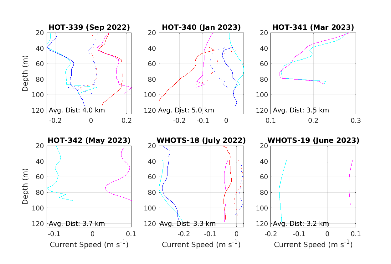
Fig. 6.38 Mean current profiles during shipboard ADCP (cyan: zonal, magenta: meridional) versus moored 300 kHz ADCP (blue: zonal, red: meridional) intercomparisons from HOT-316 through HOT-329. Moored minus shipboard ADCP differences shown in dotted lines (blue: zonal, red: meridional)
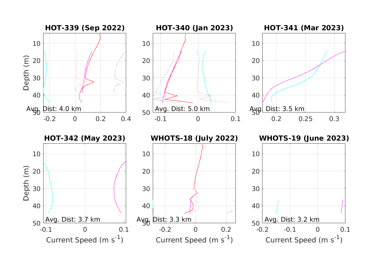
Fig. 6.39 Mean current profiles during shipboard ADCP (cyan: zonal, magenta: meridional) versus moored 600 kHz ADCP (blue: zonal, red: meridional) intercomparisons from HOT-316 through HOT-329. Moored minus shipboard ADCP differences shown in dotted lines (blue: zonal, red: meridional)
6.6. Next Generation Vector Measuring Current Meter Data (VMCM)
Time-series of daily mean horizontal velocity components for the VMCM current meters deployed during WHOTS-18 at 10 m and 30 m depths are presented in Fig. 6.40. The plots show the zonal and meridional velocity components for each depth, highlighting the variability in both east-west and north-south flows.
At 10 m depth, the zonal speed shows a notable oscillatory pattern, with peaks reaching up to 0.4 m/s in both eastward and westward directions. The meridional component at 10 m similarly exhibits variability, with alternating northward and southward flows, although the magnitude generally remains below 0.4 m/s. At 30 m depth, the zonal and meridional velocities exhibit similar oscillatory behavior, though the magnitude of the oscillations is slightly reduced compared to the 10 m depth. The zonal component continues to display alternating eastward and westward flows, with slightly dampened peaks compared to the surface. The meridional component also shows consistent fluctuations, with amplitudes generally below 0.4 m/s, indicating the persistence of dynamic current structures even at 30 m depth.
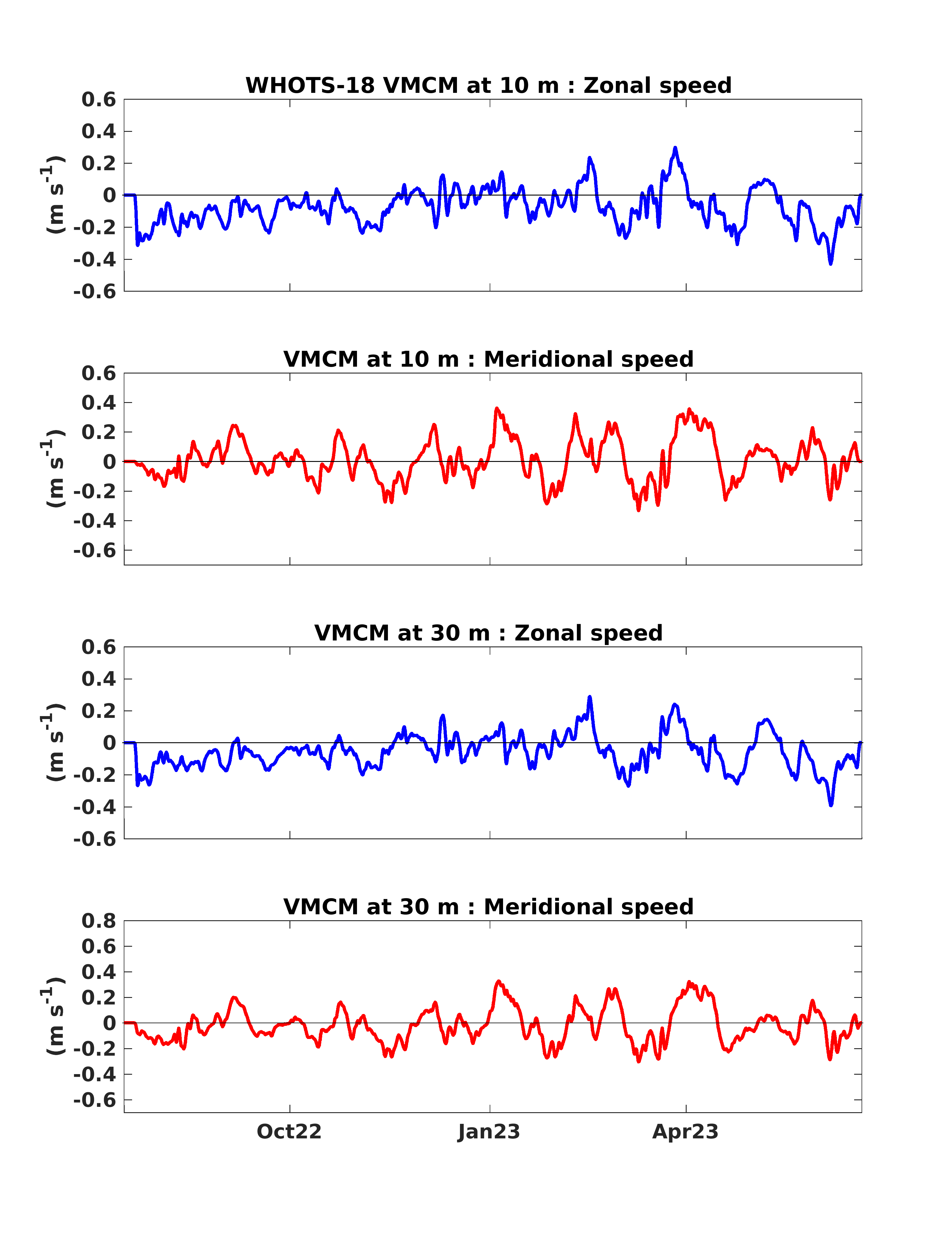
Fig. 6.40 Horizontal velocity data (\(m s^{-1}\)) during WHOTS-18 from the VMCMs at 10 m depth (first and second panel) and at 30 m depth (third and fourth panel)
6.7. GPS Data
Time-series of latitude and longitude of the WHOTS-18 buoy from GPS data are presented in Fig. 6.41. The plots illustrate the variability in the buoy’s position over time, from late July 2022 to June 2023, providing insights into the movement and stability of the buoy during the deployment.
The latitude time-series (upper panel) shows fluctuations around a central value of approximately 22.66°N, with variations ranging between 22.64°N and 22.68°N. These deviations indicate lateral movement of the buoy, potentially caused by surface currents, wind forcing, and wave action. Notable peaks in latitude variability are observed around November 2022 and March 2023, suggesting periods of increased displacement due to dynamic oceanic or atmospheric conditions.
The longitude time-series (lower panel) depicts similar variability, with values fluctuating around 157.95°W, ranging from approximately 157.92°W to 157.98°W. The longitudinal deviations mirror the behavior seen in the latitude plot, indicating that the buoy experienced both east-west and north-south drift throughout the deployment. The increased variability in longitude, particularly around November 2022 and March 2023, aligns with the latitude observations, suggesting consistent periods of elevated buoy movement.
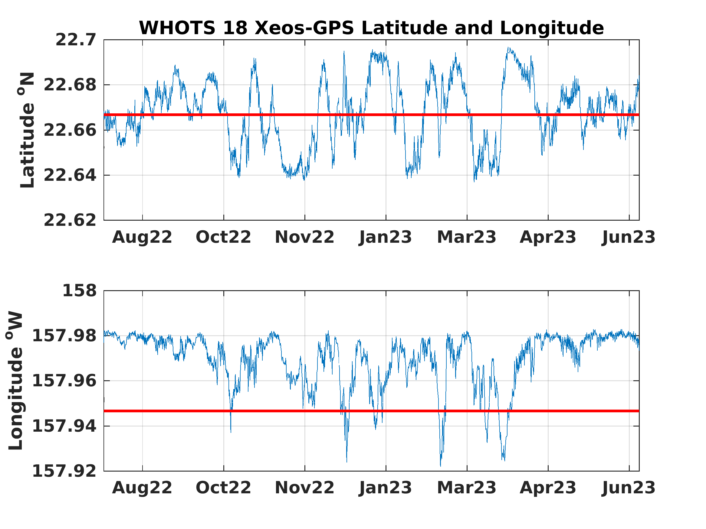
Fig. 6.41 GPS Latitude (upper panel) and longitude (lower panel) time series from the WHOTS-18 deployment.
Spectra of the latitude and longitude time-series from the WHOTS-18 buoy are presented in Fig. 6.42. These power spectra provide insights into the dominant frequencies of movement and help identify the temporal scales of variability affecting the buoy’s position.
The power spectrum of the latitude time-series (upper panel) shows a decreasing trend in energy from low to high frequencies, indicating that most of the variability in the buoy’s latitude occurs over longer timescales. The notable peaks around the frequencies marked as K1 and M2 suggest the influence of tidal components. The K1 tidal frequency corresponds to diurnal tidal cycles, while the M2 frequency is indicative of semidiurnal tides. These features highlight the impact of tidal forces on the buoy’s latitudinal movement.
Similarly, the power spectrum of the longitude time-series (lower panel) also shows dominant energy at lower frequencies, reflecting the longer-term variability in the buoy’s east-west displacement. Peaks at the K1 and M2 frequencies are also present, suggesting that the buoy’s longitudinal movement is affected by similar tidal components as the latitude. The general trend of decreasing energy at higher frequencies suggests that high-frequency processes, such as wind or short-period waves, contribute less to the overall movement compared to lower-frequency tidal and mesoscale processes.
Overall, the spectral analysis reveals that the buoy’s movement is largely driven by tidal forces, with significant contributions from both diurnal and semidiurnal components.
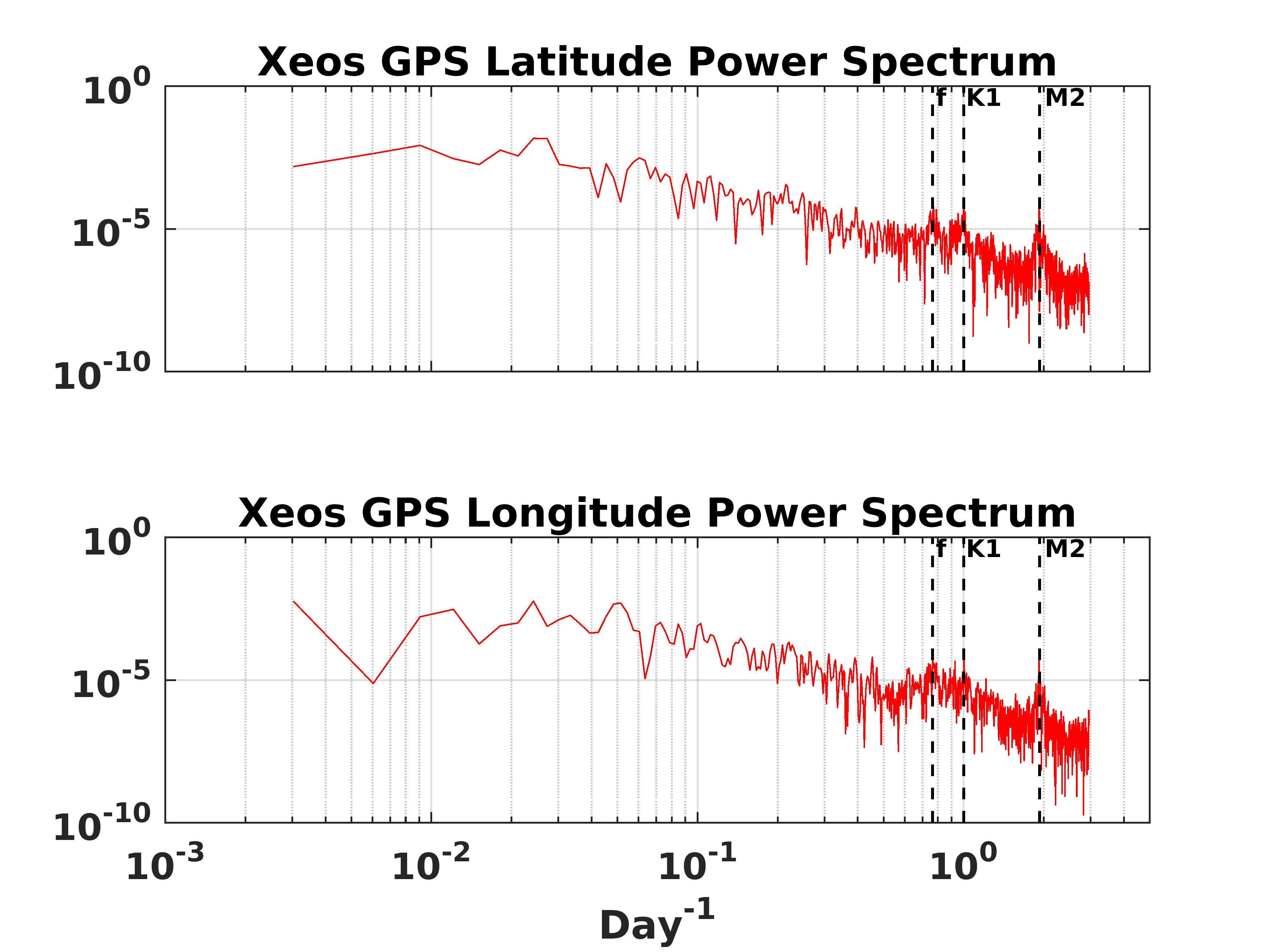
Fig. 6.42 The power spectrum of latitude (upper panel) and longitude (lower panel) for the WHOTS-18.
6.8. Mooring Motion
The position of the mooring with respect to its anchor was determined from GPS positions, supplemented by additional information provided by the ADCP data on pitch, roll, and heading. This section presents an analysis of the mooring’s motion and its relationship to the tilt recorded by the ADCP instruments.
Fig. 6.43 shows scatter plots of the ADCP tilt (a combination of pitch and roll) against the buoy’s distance from its anchor, derived from GPS positions, for both the 300 kHz and 600 kHz ADCPs during WHOTS-18. The red line in each plot represents a quadratic fit to the median tilt, calculated in 0.2 km distance bins. The plots demonstrate that as the distance of the buoy from the anchor increased, the tilt of the ADCP also increased.
This increase in tilt is consistent with the mooring line’s deviation from its vertical position as the anchor pulled on it due to environmental forces such as currents, wind, and waves. The deviation causes the mooring line to tilt, which in turn affects the attached instruments, resulting in greater tilting of the ADCPs as the buoy moves farther from the anchor. This phenomenon highlights the dynamic interaction between the mooring and its environment, which can impact the measurements taken by the instruments.
It is also important to note that both the 300 kHz and 600 kHz moored ADCPs experienced operational interruptions. The 300 kHz instrument stopped recording on January 24, 2023, and the 600 kHz instrument stopped on February 10, 2023, likely due to power loss caused by bulkhead corrosion. Despite this, the scatter plot for both ADCPs still provides valuable insight into the relationship between tilt and distance before the failure occurred. The correlation coefficients (R = 0.57 for the 300 kHz ADCP and R = 0.60 for the 600 kHz ADCP) indicate a moderate positive relationship between the distance from the anchor and the tilt, demonstrating that the farther the buoy drifted, the more significant the ADCP tilt became.
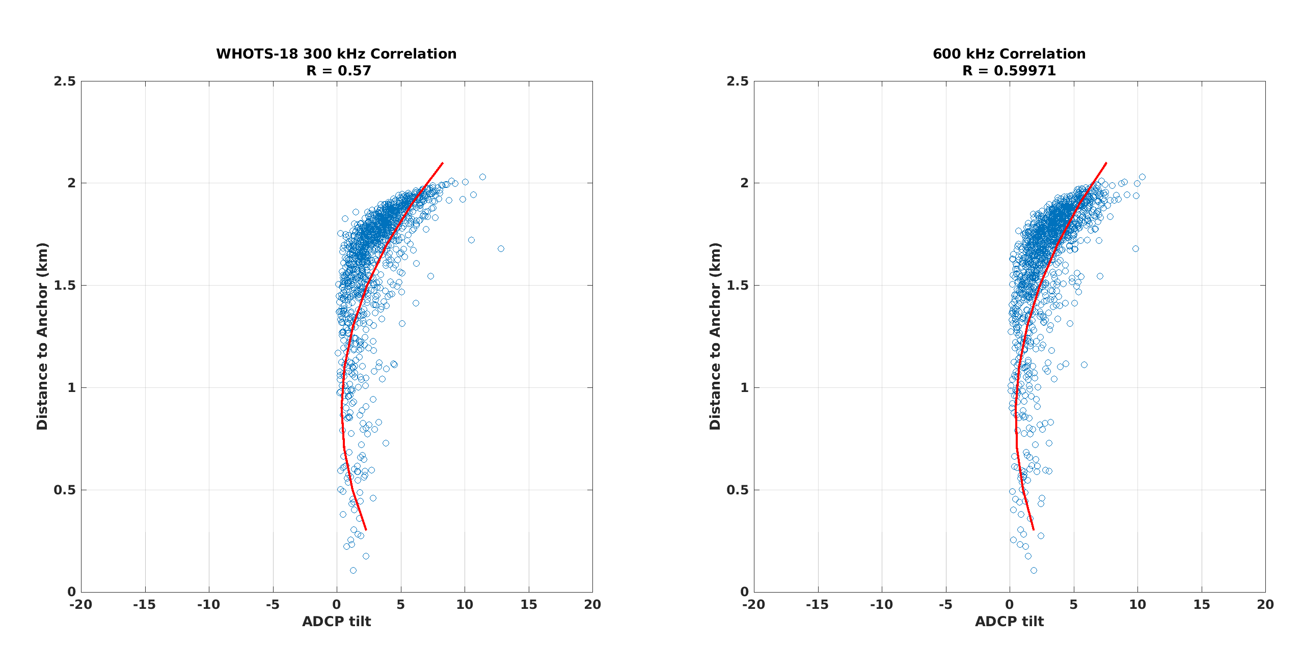
Fig. 6.43 Scatter plots of ADCP tilt and distance of the buoy to its anchor for the 300 kHz (left panel) and the 600 kHz ADCP deployments (right panel, blue circles). The red line is a quadratic fit to the median tilt calculated every 0.2 km distance bins.